(Part I)

Modeling language can be done using a wide variety of techniques (e.g. Markov chains) and in this article, we’re going to focus neural networks approaches and specifically the decoder-only architectures, which are based on the transformer architecture introduced in the paper Attention Is All You Need, in 2017. If you’re interested in it, you can read my deep dive into the architecture and the design choices here.

The decoder-only language models started with OpenAI’s paper Improving Language Understanding by Generative Pre-Training

This is a series of articles which will span:

• Part I: GPT 1, 2 and 3 (discussion on sparse transformers)
• Part II: Flagship models after GPT-4 (Llama, Mistral etc.)
• Part III: Mixture of experts and their usage in LLMs (Mistral)
• Part IV: Selective state space models and Mamba
• Extra 1: Sparse transformers

This series of article aims to dive deep in the architectural evolution of the neural networks themselves. We will also slightly focus on the training sets and approaches when deemed interesting. The first two parts are more in-tune with the evolution of the architectures and the methods while the two last parts are there to dive deep in the Mixture-of-Experts technique and the selective state space models.

I’ve also included an extra on sparse transformers. I don’t think they’re much prevalent in the LLM space but the authors of GPT-3 say that they used some ideas from that paper. I might also include more extras in the future.

The topics that will not be covered in this series of articles are:

• the other methods / techniques that have enabled such models to exist today (flash attention, multiquery attention, positional encodings such as RoPE, advances in learning rate schedulers etc.)
• Vision-Language models and Multi-Modal models in general
• alignment and what enables in-context learning, emergent properties etc., in large language models (LLMs), so everything that is RLFH, DPO etc. will not be covered
• decoding strategies
• fine-tuning (LoRA etc.)
• distillation and quantization
• model merging

Though the focus of this article is on architectural updates we’ll discuss what each paper was about and the motivations behind it. If you just want to check the specifics of each architecture feel free to jump to the corresponding section.

When considering model architectures, the specific number of layers etc. will be for the largest reported model. The global architecture stays the same across the model sizes.

GPT-1: Improving Language Understanding by Generative Pre-Training

Paper: Improving Language Understanding by Generative Pre-Training published in 2018.

Introduction and Task Modeling

GPT means Generative Pre-Training and the preprint dates back to 2018. We can already deduce that the focus will be “generative” and “pre-training”.

In statistics and machine learning, a generative model is a model of the joint probability $P(X, y)$ given inputs $X$ and outputs $y$. As opposed to a discriminative model which tries to model $P(y|X)$. You can see that with Bayes’s theorem we have a relationship between generative and discriminative models. It is generally not easy to go from a discriminative model to a generative one due to the difficulty of estimating probability densities.

How is this related to GPT-1? Well, it’s about language modeling, at least in this context, which is the task of estimating the distribution of examples $(x_{1}, ..., x_{n})$. In this case, $x_{i}$ can be a character or a word (maybe a sequence, depending on how you frame your task), generally called a token. So we’re trying to estimate $P(x_{1}, ..., x_{n})$. Thus, the generative part of it.

Note: In practice we don’t learn exactly $P(x_{1}, ..., x_{n})$ but $P(x_{n}|x_{n-1}, ..., x_{1})$.

Note: generative models existed way before transformer-based language models, see Auto-Encoding Variational Bayes and Generative Adversarial Networks (2014). See Denoising Diffusion Probabilistic Models (2020) for other generative models.

The “Pre-Training” part in the GPT name comes from using a large dataset of unlabeled textual data to first train the model to a certain performance. This phase is the pre-training phase. Then the model would be used on “downstream” task, to fine-tune it on supervised datasets. The authors describe this as a semi-supervised approach, combining an unsupervised pre-training of the model and a supervised fine-tuning of it. It’s a two-stage procedure.

The idea of doing so comes the abundance of unlabeled data in NLP and the difficulty and cost of creating good supervised datasets. This approach though, has some great benefits. By learning on a varied training set which would span a lot of different topics, contexts etc., the model learns good and robust representations that can boost its performance when later on fine-tuned on a supervised dataset as found in the paper Why Does Unsupervised Pre-training Help Deep Learning? (according to the authors, pre-training acts as regularization allowing better generalization of deep neural networks)

Albeit these benefits, this approach poses two challenges specific to it, and a third challenge due to the architecture used in this context:

The first one is finding a good optimization objective to use so that the learned representations transfer well to the downstream tasks. It should be such that the pre-training provides a nice initialization point for fine-tuning.

The unsupervised pre-training objective here is about maximizing the following likelihood:

$$L_{1}(x) = \sum_{i}^{}{log\Bigl(P(x_{i}|x_{i-k},…,x_{i-1};\Theta)\Bigr)}$$

Where $\Theta$ represents the parameters of our model. This stems from decomposing the previous joint probability into the product of conditional probabilities $p(x)=\prod_{i}^{}{p(x_{i}|x_{i-k},…,x_{i-1})}$, for which the log-likelihood is more approachable to optimize.

The probabilities in this case are produced by the last softmax.

The authors use the following notation to denote the equations in GPT-1:

$$\begin{matrix} h_{0}=UW_{e} + W_{p}\\ h_{l} = transformer\_block(h_{l-1}), \forall i \in [1, n]\\ P(u) = softmax(h_{n}W_{e}^{T}) \end{matrix}$$

$W_{e}$ is the encoding matrix. As we can see, they use the same trick as in the original transformer paper where the last linear layer shares the same matrix as the encodings. $W_{p}$ are the positional encodings. Them being at this stage means that they’re absolute position encodings. (You can read more about that on my blog post about transformers)

The second challenge is the optimization objective of the downstream task. Following in the steps of previous approaches the authors use an auxiliary unsupervised objective along the supervised one. Though they found that the text representations learned through unsupervised pre-training already contain linguistic aspects relevant to the target tasks, they still used the language model objective as an auxiliary one.

The supervised learning optimization is thus the combination of the language modeling loss function $L_{1}$ and a loss function specific to the supervised part $L_{2}$. So the real loss function here is $L_{3}(C) = L_{2}(C) + \lambda L_{1}(C)$.

$$ L_{2}(C) = \sum_{(x, y)}^{}{logP(y|x^{1}, …, x^{m})}$$

Where $logP(y|x^{1}, …, x^{m}) = softmax(h_{n}^{m}W_{y})$ with $W_{y}$ being the linear layer added on top of the transformer.

The third challenge is adapting the architecture to the downstream tasks while making minimal changes. The solution to this issue is to use “task-aware” input transformations. Since the model trained on contiguous sequences of text and since some tasks are formulated in a specific way, one should take into account these transformations during the fine-tuning.

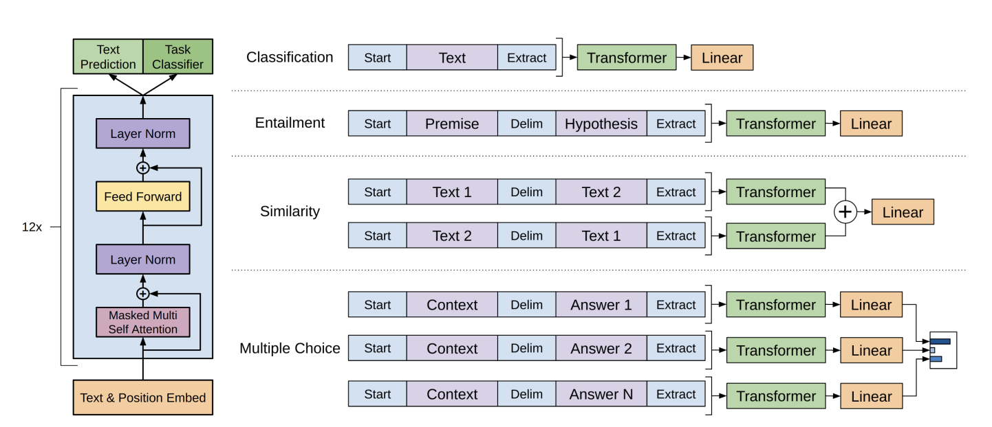
As you can see here, on top of the added (linear + softmax) layer, the authors use special tokens for each task. The special start <s> and extract <e> tokens are randomly initialized. Nothing is said about the delimiter token ($) but it’s safe to assume it’s randomly initialized as well.

The linear and softmax layers’ roles are clear for the classification and entailment tasks. For the similarity task each combination is processed independently by the model, which gives us two outputs, these are summed up together and fed to the linear layer. For the multiple choice task, each combination is processed independently as well then fed to the softmax, so $softmax(\sum_{choices}^{}h_{n}^{m_{choice}}W_{y})$.

Architecture and Training

Dataset:
BooksCorpus dataset: contains long stretches of contiguous text, which allows the model to learn to condition on long-range information. The dataset was cleaned and standardized using the spaCy tokenizer.
(they also trained on Word Benchmark which is shuffled at the sentence level destroying the long range structure)

Tokenizer:
BPE (Byte-Pair Encoding) with 40000 merges

Neural Network Architecture:

• Positional encoding: learned
• Transformer-based, decoder only
• Number of layers: 12
• Model dimension: 768
• Number of heads: 12
• Type of heads: masked, dense/full, self-attention (all of them, crucial for maintaining the auto-regressive property)
• Intermediate size (point-wise feed-forward network dimension): 3072 (the classic model dimension * 4)
• Weight initialization: Normal with $0$ mean and $0.02$ standard deviation. (I didn’t find why exactly this initialization scheme maybe it’s because layer norm normalizes affects inputs to the layers, it stabilizes their mean and their variance which makes the model less sensitive to initial weights. The exact number may have been found empirically)
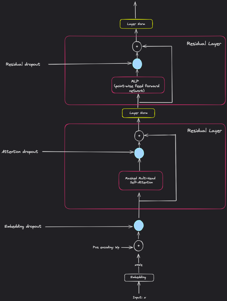
• Dropouts: (see the figure below to understand where the dropouts are placed)
  • Residual: 0.1
  • Embedding: 0.1
  • Attention (can also be called residual I guess): 0.1
• Activation function: GeLU

Optimization scheme:

• Optimizer: AdamW
• Max learning rate value: 2.5e-4
• Learning Rate Scheduler:
  • Type: Linear increase + cosine annealing
  • Strategy: Increase from 0 to 20 000 then annealed to 0
• Regularization: L2 with $w=0.01$ on all non-bias and non-gain weights (I believe gain weights refer to the scaling factors in normalization layers)

Training:

• Context size: 512
• Number of epochs: 100
• Sampling strategy: random
• Batch size: 64

Finetuning:

For most tasks:

• Added Dropout to the classifier: 0.1
• Learning rate decay with warmup over 0.2% of the training set and $lambda=0.5$. For most tasks though the learning rate is fixed (I believe) at 6.25e-5.
• Batch size of 32
• 3 epochs of fine-tuning were sufficient for most cases.

GPT-2: Language Models are Unsupervised Multitask Learners

Paper: Language Models are Unsupervised Multitask Learners published in 2019.

Introduction

The goal here is to double down on the unsupervised learning setting and how it enables learning tasks without any explicit supervision training. The goal here is to achieve a reasonable performance in a zero-shot task transfer through and the main way to achieve that will be scaling up the model. Zero-shot transfer here means to use only use what the model learning during the unsupervised training to solve a task (The section about GPT-3 delves into the details of meta learning, in-context learning, zero-shot learning and few-shot learning). The authors say that with supervised training we obtain “narrow experts” that are sensitive to data shift rather than “competent generalists”.

Such a generalist system should be able to perform many different tasks, so it should learn to model the conditional probability distribution $p(.|input, task)$, as opposed to performing a single task which requires us to model $p(output|input)$, now we have to condition on the task as well. This task conditioning is often implemented at an architectural level or at an algorithmic level (optimization and training specification etc.).

The authors have an interesting hypothesis following this; language modelling enables us to learn the different tasks of language without explicitly introducing the conditioning. Their idea is that learning a specific language task in a supervised setting requires specifying the input and output examples in a specific manner, and this is only a subset of all the examples that we’re learning on in a an unsupervised setting. So optimizing a language supervised objective is the same as optimizing the unsupervised objective but evaluated on a subset of examples. The global minimum of the unsupervised objective is also the global minimum of all supervised objectives.

That hypothesis can be framed equivalently by saying that a language model with sufficient capacity will learn tasks illustrated through natural language sequences as part of improving its prediction capabilities, irrespective of how these tasks are obtained. Succeeding in this is succeeding in unsupervised multitask learning. The authors evaluate that by evaluating the zero-shot capabilities on a wide variety of tasks.

Architecture and Training

Training set:
WebText. A dataset created from scraping web pages obtained through outbound links from Reddit when users have at least 3 karma. They excluded links created after December 2017, removed duplicate documents and Wikipedia content, and applied heuristic-based cleaning. Over 8 million documents totaling 40 GB of text were included after preprocessing.

Tokenizer:
Byte-level BPE with two rules:
1/ prevent from merging tokens across different character categories within byte sequences
2/ spaces are exempt from the first rule because this way we obtain better compression efficiency and we minimizes the fragmentation of words across multiple vocabulary tokens

Vocab size: 50 257

Note on BPE:
The authors said some interesting stuff about BPE so I thought of including it here for completeness.
Why BPE? BPE is falls in the middle ground between character-level and word-level language modeling. It uses frequent symbol sequences as word-level inputs and infrequent symbol sequences as character-level inputs, so we have a better trade-off between vocabulary size and capturing linguistic information.
Why byte-level? FIrst, it’s not because BPE is called Byte-Pair Encoding that the default/reference implementations are on bytes. The authors prefer a byte-level BPE (so the same logic of algorithm but applied to bytes) because it reduces significantly the vocabulary size and only requires a base vocab size of 256. This is also cool because now we won’t require some kind of specific or lossy pre-processing or tokenization and the model can be evaluated on any benchmark as it is.
Why add the rules? BPE using a greedy frequency based heuristic for building the token vocabulary, applying it directly to the byte sequence results in sub-optimal merges. Like dog, dog., dog?, are considered different tokens while they’re just variations of the same word. “This results in a sub-optimal allocation of limited vocabulary slots and model capacity”. So a rule was added to prevent from merging different character categories (letters and punctuation for example). This rule doesn’t concern space because we still want to have a merge like the ,or while the, etc. because it’s common across the corpus thus “improving compression efficiency while adding minimal fragmentation of words across vocab tokens”.

Neural Network Architecture:
Positional encoding: learned
Transformer-based, decoder only
Number of layers: 48
Model dimension: 1600
Type of heads: masked, dense/full, self-attention
Number of heads: not mentioned (only for the smallest model in the official code)
Intermediate size: 6400 (not explicitly mentioned, but in the official code we see that it is equal to model dimension * 4)
Layer normalization position: pre (see the figure below)
Weight initialization: They don’t mention weight initialization for every weight and bias but they say that they scale the initialization of the weights of the residual layers by $\frac{1}{\sqrt{N}}$ where $N$ is the number of residual layers (so $2 * num\_layers$ because each block layer contains two residual layers). They use “model depth” in this scaling to “account for the accumulation on the residual path”.
Dropout: exact value not mentioned, but see the figure below to understand the positioning
Activation function: GeLU

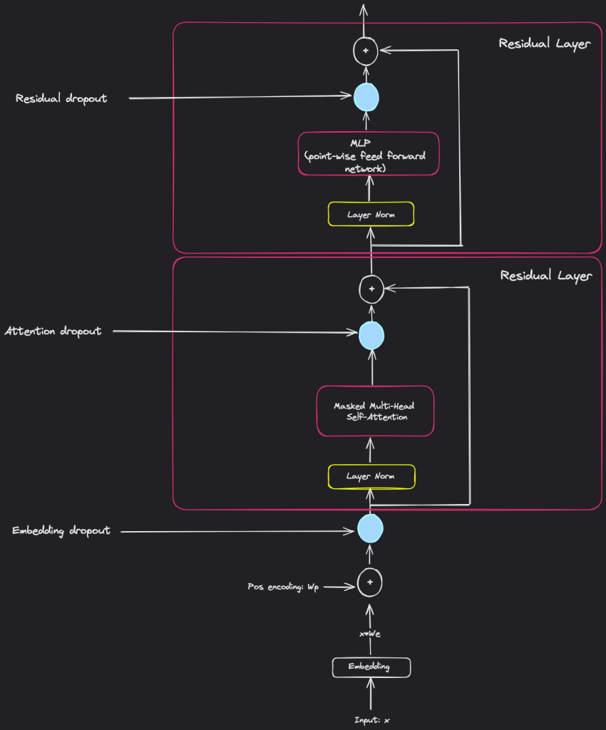
Note about the pre-layer norm and weight initialization scheme in residual layers:
The usage of layer normalization at the beginning of the residual layers resembles the pre-activation residual networks from Identity Mappings in Deep Residual Networks. The authors say that their weight initialization scaling was done to “account for the accumulation on the residual path”. So residual paths help mitigate the vanishing gradients problem in deep neural networks since they offer alternative paths for the gradient during backpropagation. Why we need that initialization scaling? So how I understand it is that by adding more layers, their outputs will accumulate along these residual paths and if not properly handled this accumulation can lead to gradients that are either too large (maybe too small as well but I’m not sure).So that’s why the scaling uses the number of residual layers, and by reducing the scale of weights we ensure small initial weights which helps us avoid large initial gradients after passing through many residual layers. This will make the training more stable.

Optimization scheme:
The learning rate was manually tuned for the best perplexity on a 5% held-out sample of WebText.

Training:
Context size: 1024

GPT-3: Language Models are Few-Shot Learners

Paper: Language Models are Few-Shot Learners published in 2020.

Introduction

As the name of the paper suggests, the goal is to demonstrate that large language models are capable of in-context learning. Having models capable of that is great because the previous two-stage procedure of pre-training a model on large unlabelled corpus of text then fine-tuning requires good, sufficiently large, task-specific supervised datasets for the fine-tuning.

If we’re capable to include task-specific knowledge in the prompt of the model instead of going through the fine-tuning phase we’d bypass the need for this qualitative and costly task-specific datasets.

This property not only solves the difficulty of collecting datasets for each new task but also the possibility of exploiting spurious correlations in the collected fine-tuning datasets. The potential to exploit spurious correlations in training data fundamentally grows with the expressiveness of the model and the narrowness of the training distribution. This can happen in the two-stage procedure because we need a very large model to absorb all of the information from the pre-training dataset but then we fine-tune it on a narrow task-specific dataset, which definitely hurts the generalization of the model since it picks-up the noise from the specific dataset as well. There are many papers about the generalization capability of models and its relationship with the variance in the training datasets, the model size, theoretical extrapolation results etc., but the authors mention two specific papers in thise case for those that want to read them, Learning and Evaluating General Linguistic Intelligence and Right for the Wrong Reasons: Diagnosing Syntactic Heuristics in Natural Language Inference.

The authors also mention the fact that humans do not require large supervised datasets to learn most language tasks and it allows them to mix tasks and fluidly switch between different tasks without having their performance degraded. So this is also a motivation behind scaling up GPT-3 to its $175$B size. Not only it must not need to be fine-tuned for every tasks, but to give it the capability for the same model to “recognize” and “deal” with many tasks even if they’re mixed in the same text.

The paper shows that scaling up language models in the context of meta-learning greatly improves task-agnostic, few-shot performance, sometimes even reaching competitiveness with prior state-of-the-art fine-tuning approaches. Let’s see what meta-learning is about.

Meta-Learning, In-Context Learning, 0-Shot, Few-Shot, Fine-tuning

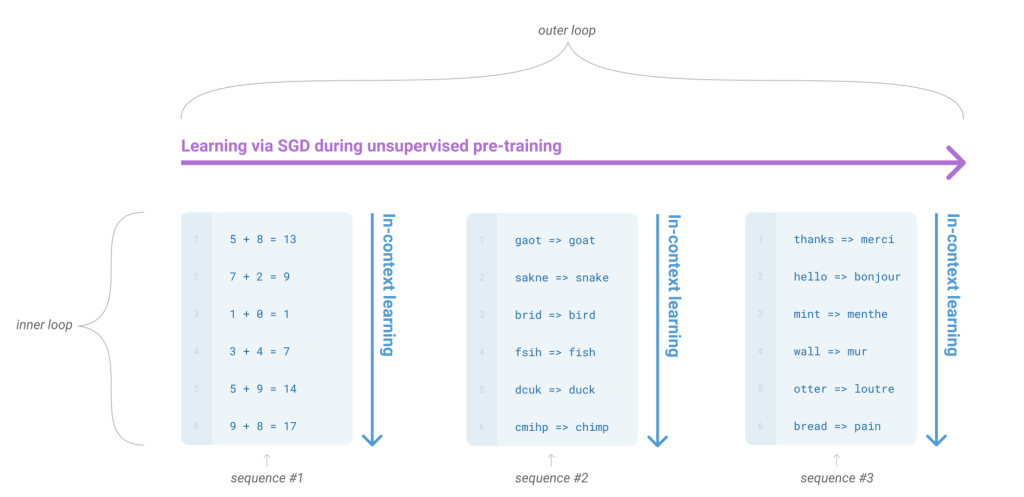
Meta-learning is a two-step procedure involving two loops, one “inner-loop” and one “outer-loop”. Meta-learning can be seen as “learning to learn”. In our case, of language models, we want the model to develop a broad set of skills and pattern recognition abilities during the training phase that can later be utilized for various tasks at inference time without having to fine-tune it. The “outer-loop” is the training with gradient updates (that’s typically done with Adam optimizer etc.) where the model acquires general capabilities, whereas in the “inner-loop” the model uses these capabilities to handle specific tasks.

Personal note: I think the dataset (a part of it I guess) is formatted in such a way where the model tries to exhibit its capabilities in the inner loop, which is a forward pass, and at the outer loop it learns what it needs to learn (where it failed). This way we don’t need further gradient updates or training for the downstream tasks. But this supposes that the labeled dataset contains a wide variety of tasks. So, I think the goal here is to make the model capable of learning from the context itself rather than learning a wide variety of fundamental tasks through this meta-learning specification/formulation in the hopes of it generalizing to unseen tasks that would span from these fundamental tasks.

As you can see in the figure, in-context learning is used during the inner loop of meta-learning. The language model uses the context provided to perform the related tasks. It’s like it’s “learning from the context”. This is in the inner loop so we’re using the model’s previously trained capabilities to generate predictions that align with the new context it encounters.

Zero-shot learning is the capability of the model to perform tasks using only its pre-trained knowledge, without any examples in the context and without any fine-tuning on that task. So even though it’s called “zero-shot,” the model, often, has seen the type of task during its pre-training, but, probably not, the specific instance or variation of the task it encounters during inference. This is a fundamental concept when it comes to the generalization capabilities of learning models, allowing them to apply broad knowledge to new scenarios without additional training.

Few-shot learning is kind of an “extended” case of zero-shot learning where the model is provided with a few examples of a specific task in its context during inference. This method lies between zero-shot learning, where no examples are provided, and fine-tuning, where the model undergoes additional training. Few-shot learning is used a lot on to improve the model performance without fine-tuning.

I’m sure that you’re familiar with fine-tuning, but just in case, it is the additional training on top of a pre-trained model, usually with a dataset specific for a particular task or domain. The goal is to have a nice initialization point during the optimization of the weights to slightly adjust them in the correct directions, thus refining its abilities to perform better on tasks that require specialized knowledge beyond its initial training.

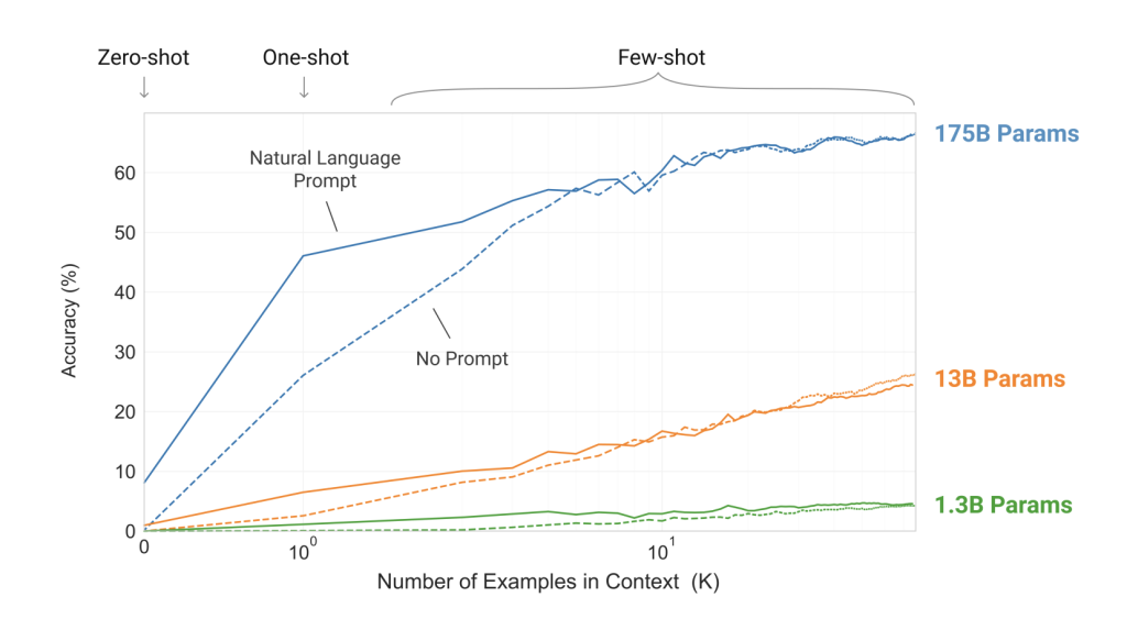
The figure above is for the task of removing random symbols from a word. There are more details about the task in the figure. The x-axis shows the number of examples provided in the context on a logarithmic scale. The y-axis measures the accuracy of the task, which in this case is removing random symbols from a word. The figure shows the performance of different scales of the model with respect to the number of examples in the context. It also shows the case where we give a prompt (to guide the model on this task), which means we specify the task in textual language (and we include the examples) and when we don’t, in this case we just give the input and expected output (the examples) directly.

• Scaling up the language model increases the accuracy whether we’re using a prompt to specify the task or not.
• The few-shot performance is better than the one-shot performance which is also better than the zero-shot performance.
• Accuracy increases with the number of examples in the context.
• Prompting the model helps, unless the number of examples in the context is very large (more than a thousand). In this case the performance is nearly the same between prompting the model and just giving it the examples.

Note: the goal of this article is not to delve deep into which tasks GPT-3 was better on with which non-gradient involving technqiue versus with fine-tuning. The figure above is just representative of the evolution of the accuracy on a task with respect to the different techniques of in-context learning. I have included it because most of the model exhibit the same behaviour. The ability to perform better or not on a task with fine-tuning will depend a lot on the specific model, how it was trained, the training set, the fine-tuning set etc.
The goal of this article is to focus on architectural updates while discussing what each paper was about.

Architecture and Training

Dataset selection

The following describes the training set selection methodology:

Initial dataset:

• Primary source: Common Crawl, which is a large-scale web corpus, constituting nearly a trillion words at the time. It is vast and diverse upon which you can train a large model like GPT-3 (175B) without repeating data sequences, but at the same time it contains a lot of low quality data. The authors took two steps to improve the quality from the Common Crawl, but also added high-quality datasets in the training set.
• Datasets to augment the primary source: quote from the paper: “several curated high-quality datasets, including an expanded version of the WebText dataset [RWC+19], collected by scraping links over a longer period of time, and first described in [KMH+20], two internet-based books corpora (Books1 and Books2) and English-language Wikipedia.”

Improved dataset:
Two approaches were taken to improve the quality of the Common Crawl:

• Quality Filtering Using a Classifier:
  • Use a classifier trained to distinguish high-quality text (positive examples) text from low-quality text (negative examples) to resample the Common Crawl and keep samples that the classifier deemed of high-quality.
  • Positive examples: a collection of curated datasets such as WebText, Wikiedia, and the web books corpus
  • Negative examples: unfiltered Common Crawl
  • Features: features from Spark’s standard tokenizer and HashingTF
  • Selection process:
    • Pareto distribution: $\mathrm{np.random.pareto}(\alpha) > 1 - \mathrm{document\_score}$
    • $\alpha$ choice: It was chosen to match the distribution of scores from the classifier on WebText, whcih gave $\alpha = 9$
• Fuzzy Deduplication at the Document Level, done for each data set and to remove WebText from Common Crawl
  • Document processing: same features as to train the classifier above, which means Spark’s standard tokenizer and HashingTF
  • Producing MinHashes:
    • The features of a document are used to produce hash values
    • Number of hash functions: 10
    • We select the minimum across to get the MinHash signature
  • Bucketing with Locality-Sensitive Hashing (the threshold is not mentioned)

Decontaminated dataset:

• Documents shorter than 200 characters are discarded.
• For each document:
  • 13-Gram Search: search for overlaps of 13 consecutive words (grams) between the test/development sets and the training data. A gram was defined as a lowercase word delimited by whitespace, without punctuation.
  • If a 13-gram overlap was found:
    • Removing Contaminated Segments: when a 13-gram overlap was found, a 200-character window around the overlapping text was removed from the training dataset. Split the document here.
    • Repeat this step until either:
      • The document is split 10 times, in which case it is discarded because deemed too contaminated. Originally the authors used a single collision rule but they found that too many documents were flagged as positives falsely because for example Wikipédia articles would quote lines from books, or there are adages and proverbs that are repeated across documents but we want the model to learn them because it’s supposed to be common knowledge etc.
      • Otherwise it is kept

Final dataset:
The final training dataset is a mixture of the different data sets after all the quality filtering, deduplication and decontamination:

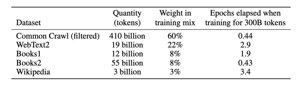
This is an important table to understand. First, all GPT-3 models (all sizes) were trained for a total of 300 billion tokens. We can see that the Common Crawl alone is larger than that.

There are three things that should be known / understood:

• The sampling from each dataset: the authors said that sampling was not done in proportion to the data sets, but rather according to the perceived quality, so data sets like CommonCrawl and Books2 are sampled less than once during training, but the other datasets are sampled 2-3 times.
• Weight in training mix.
  • The authors say that it’s the fraction of training data that comes from the data set. It is intentionally not proportionate to the size of the dataset.
  • E.g. 60% of the 300B seen during training come from the Common Crawl, which represents 180B tokens.
• Epochs elapsed when training for 300B tokens.
  • It is an indicator of how many times, on average, the model sees a particular example from the dataset during its training.
  • E.g., 2.9 from WebText2 means that the model sees the same example almost three times during training. The authors prefer a slighly overfitting in exchange for higher quality data during training.

During training they packing multiple documents into a single sequence when documents are shorter than $2048$ because the context window used is $2048$. When many documents are present in the same sequence, they use a special end of text token to separate between them instead of using some kind of masking. This is more efficient during training and the model will pick up the meaning behind that special token as the documents it separates are unrelated.

Architecture

The authors give the configurations for the different sizes:

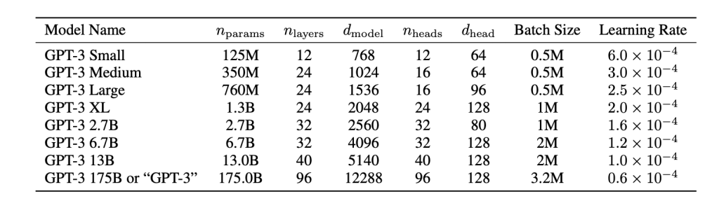
The tokenizer is the same for all models.

We’ll focus on GPT-3, which refers to the model with 175B:

Note:
The information below certainly doesn't represent the real GPT-3 model as developed by OpenAI. The code for it and the weights are not publicly available. I'm inferring the architecture from what is said in the paper. For example we don't know how they alternated dense and sparse attention patterns or which sparse patterns they have used. We also don't know exactly if there is a particular weight initialization method that was used etc. The same goes for the exact sampling probabilities used, the exact batch size at each step etc.

Tokenizer:
Same as GPT-2 with the reversible tokenization as well

Neural Network Architecture:

• Positional encoding: same as GPT-2
• Transformer based, decoder-only, usage of alternated dense and locally banded sparse attention patterns, as in the paper Generating Long Sequences with Sparse Transformers (read my post about it)
• Number of layers: 96
• Model dimension: 12288
• Number of heads: 96
• Type of heads: sometimes dense masked self-attention heads, and sometimes a masked sparse self-attention head
• Intermediate size: 4 * $d\_model$ = 49152
• Weight initialization: Same as GPT-2
• Dropouts: Same as GPT-2
• Activation function: Same as GPT-2

It’s hard to know the exact architecture because the authors didn’t specify how they alternated the dense and locally banded sparse attention heads (but I guess each dense layer is followed by a sparse layer), they didn’t specify the exact sparsity patterns used (the paper referenced introduces two mains patterns “strided” and “fixed”, and mentions that “fixed” is more suited for language tasks), they also didn’t specify how the sparse heads were used, does the $d\_heads = 128$ concern both the dense attention layers and sparse attention layers or only the dense layers? If it concerns both, did they use for the sparse attention layer a “merged” head approach as described in the reference paper or a multi-head approach. And if it’s not, did they apply exactly the same sparsity pattern across all the heads or did they try to connect every output to every input across these heads? You can learn about the sparse transformers in my blog post here.

Optimization scheme:

• Optimizer: AdamW, $\beta_{1}=0.9$, $\beta_{2}=0.95$, $\varepsilon=10^{-8}$
• Gradient clipping: yes
  • Strategy: clip the global norm of the gradient at 1.0
• Starting learning rate value: 0.6e-4
• Learning Rate Scheduler:
  • Learning Rate Warmup: Linear, over the first 375M tokens
  • Cosine Decay: gradually reduced to 10% of its initial value over 260B tokens
  • Post-Decay:continues at 10% of its initial value for the rest of the training
• Regularization: $w=0.1$

Training:

• Context size: 2048
• Batch size: Batch size is increased linearly from a small value (32k tokens) to the full value (3.2M tokens) over the first 4-12 billion tokens of training, depending on the model size. They also say that they guided their choice of the batch size by measuring the gradient noise scale during training as was done in the paper An Empirical Model of Large-Batch Training
• Samplig: As explained before, each dataset is sampling with a different frequency, sampling is done without replacement within an epoch