On this page
I was qualifying exact checkpoint resumption for a Qwen3.5-0.8B Base training path in Open-Instruct. This was not a single-GPU save-and-load test. The model ran on one node with four A100-SXM-64GB GPUs under PyTorch DistributedDataParallel. Each optimizer update consumed eight packed sequences of 32,768 tokens: one sequence per rank for two gradient-accumulation microbatches, or 262,144 tokens globally. Forward and backward used BF16 autocast while parameters, gradients, and AdamW moments remained FP32.
I trained one branch continuously from updates 1 through 10. After update 5, I wrote a full checkpoint. I then launched a fresh four-rank process group, rebuilt the model, optimizer, scheduler, trainer, and DDP wrappers, restored that checkpoint, and reran updates 6 through 10 over the exact same packed examples.
The target was not “roughly the same curve.” I wanted exact counterfactual continuation:
If interruption had never happened, would every subsequent training state have been identical?
At first, the checkpoint appeared perfect. The model parameters were exact. The optimizer state was exact. The scheduler, trainer counters, Python RNG, NumPy RNG, CPU Torch RNG, and every CUDA RNG stream were exact. The resumed process consumed the same token IDs, the same supervised positions, the same packed examples, and the same number of tokens.
The loss reported below is the token-normalized training objective over the globally supervised target positions across all four ranks. At the first resumed update, both branches produced exactly the same forward loss:
continuous update 6 loss = 0.8891351451286653
resumed    update 6 loss = 0.8891351451286653
Then update 7 disagreed:
continuous update 7 loss = 0.7142631975696954
resumed    update 7 loss = 0.7143024200392002
absolute difference       = 0.00003922246950482977
By update 10, one embedding tensor differed in 164,523,523 of its 254,279,680 FP32 elements. That is 64.7017972494 percent of the tensor. Its maximum absolute difference was only 1.7233192920684814e-05, but the resumed execution was no longer the same execution.
The instinctive diagnosis was “NCCL nondeterminism.” That diagnosis was too vague to be useful and, at one point in the investigation, wrong. I eventually found three distinct pieces of process state that a conventional training checkpoint did not capture:
- a causal-convolution backward path that used unordered CUDA atomics
- per-process Triton autotune choices interacting with a shared disk cache
- the age-dependent bucket topology of PyTorch DistributedDataParallel’s reducer
Fixing the first two made every rank-local gradient exact. Training still diverged. The remaining difference appeared only after DDP reduced those exact gradients. The continuous process had 61 gradient buckets. The fresh resumed process had one.
I wanted to know exactly where the two runs stopped being the same. That meant looking past the checkpoint load itself and comparing what each fresh process did during the next training update.
The claim, and its deliberately narrow scope
The experiment in this post used one text-only Qwen3.5-0.8B Base model inside a pinned Open-Instruct training path, on one node with four A100-SXM-64GB GPUs. It used PyTorch 2.9.1+cu129, dynamic DDP, BF16 autocast, FP32 parameters and gradients, gradient accumulation of two, and fused AdamW.
Within that system, I established the following:
Restoring all checkpointed training state did not produce exact continuation because numerically relevant process-local runtime state was reconstructed differently. Once I made the causal-convolution path deterministic, froze the executed Triton autotune records, and initialized both DDP reducers to the same mature bucket layout before either branch processed its next training batch, continuous and resumed training matched exactly through update 10.
This is not a claim that NCCL is broken. It is not a claim that every DDP job has this failure. It is not evidence about FSDP, tensor parallelism, context parallelism, HSDP, multiple nodes, another PyTorch version, another optimizer, or another Qwen3.5 implementation.
I do not know how often this exact reducer mismatch appears in other training stacks. I am sharing it because the debugging method is broadly useful: when a resumed run drifts, compare the boundaries in order and include runtime state, not just checkpoint contents. The 61-bucket versus one-bucket mismatch is one example of the kind of state an ordinary restore check will never see.
Resume equivalence is larger than checkpoint equivalence
Let the persistent training state after update \(t\) be \(P_t\). It includes the state I normally expect a serious checkpoint to contain:
\[ P_t = (\theta_t, O_t, S_t, R_t, D_t, M_t) \]where \(\theta_t\) is model state, \(O_t\) optimizer state, \(S_t\) scheduler and trainer state, \(R_t\) random-number-generator state, \(D_t\) data position, and \(M_t\) any other serialized metadata required by the trainer.
Let \(X_{t+1}\) be the exact rank-local training input for the next update. A useful but incomplete model of resumption is:
\[ P_{t+1} = T(P_t, X_{t+1}) \]Real training code has another input: process-local execution state \(E_t\). It includes selected kernel algorithms, autotune results, compiled graphs, communication topology, DDP reducer buckets, allocator history, and other state reconstructed after process launch.
\[ P_{t+1} = T(P_t, X_{t+1}; E_t) \]Exact continuation therefore requires more than \(P_t^{(c)} = P_t^{(r)}\) and \(X_{t+1}^{(c)} = X_{t+1}^{(r)}\). At every numerically relevant boundary, the continuous process state \(E_t^{(c)}\) and resumed process state \(E_t^{(r)}\) must be equivalent for the transition being computed.
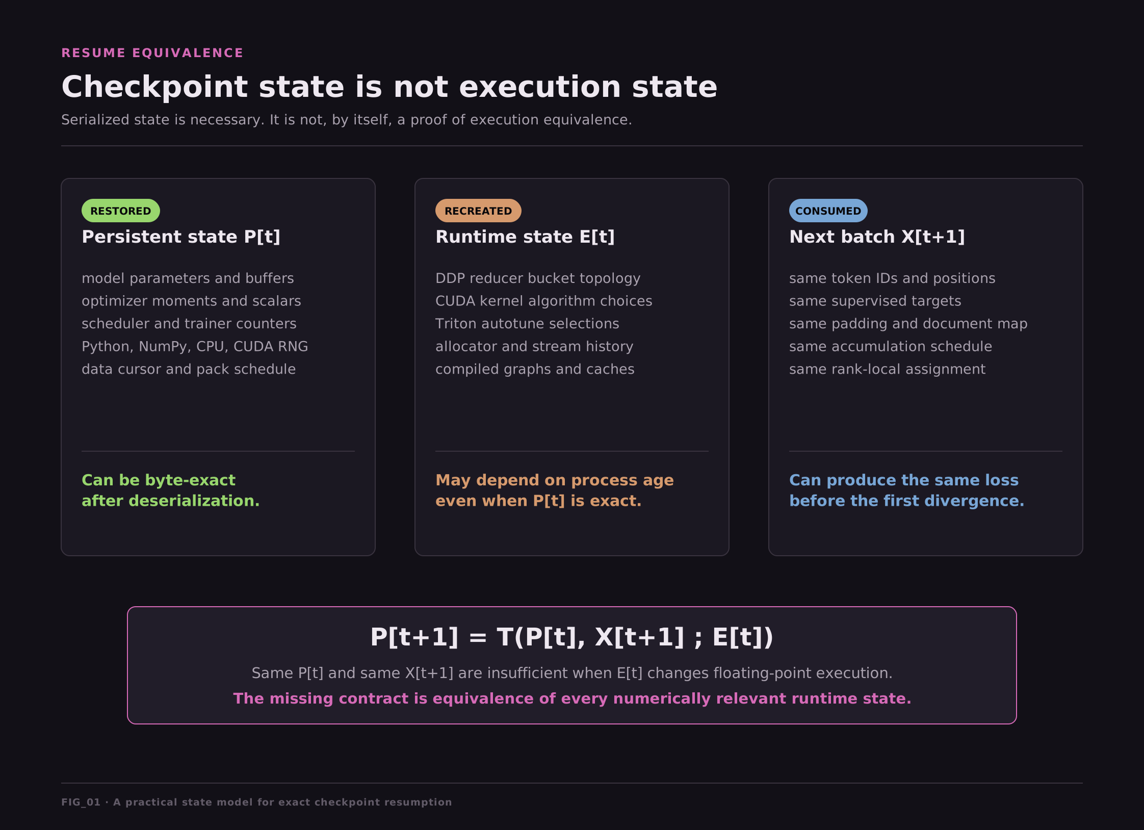
A load test proves that state can be deserialized but it does not prove that a fresh process will execute the next update identically to a process that has already executed five updates.
The branch experiment
I wanted a real process boundary, not save and load inside one Python process. The experiment had two legs:
continuous:  fresh launch → updates 1, 2, 3, 4, 5 → updates 6, 7, 8, 9, 10
                                             ↓
                                      checkpoint 5
                                             ↓
resumed:                                fresh launch → restore → updates 6, 7, 8, 9, 10
The resumed leg started new rank processes and constructed new model, optimizer, scheduler, trainer, and DDP objects. It then restored the checkpoint taken from the continuous leg. Both legs consumed the same precomputed packs for updates 6 through 10.
The fixed geometry was intentionally small enough for forensic repetition and large enough to exercise the full training path:
| Dimension | Frozen value |
|---|---|
| Model | Qwen3.5-0.8B Base, text-only converted checkpoint |
| Model revision | dc7cdfe2ee4154fa7e30f5b51ca41bfa40174e68 |
| Trainable state | 320 FP32 tensors, 752,393,024 elements |
| Hardware | one node, 4 × A100-SXM-64GB |
| Parallelism | pure dynamic DDP, world size 4 |
| Sequence length | 32,768 tokens |
| Microbatch | 1 packed sequence per rank |
| Gradient accumulation | 2 microbatches |
| Tokens per optimizer update | 262,144 fixed tokens |
| Data | 80 packs, no reuse, 10 updates |
| Precision | BF16 autocast, FP32 parameters, gradients, and AdamW moments |
| Optimizer | fused AdamW, β₁ 0.9, β₂ 0.95, ε 1e-8, weight decay 0.1 |
| Schedule | 2e-5 peak learning rate, cosine decay, 3% warmup over the frozen horizon |
| Gradient clipping | global norm 1.0 |
| DDP bucket cap | 25 MiB |
| Activation memory | non-reentrant gradient checkpointing enabled, Liger disabled |
| Core runtime | PyTorch 2.9.1+cu129, Transformers 5.14.0.dev0, Accelerate 1.12.0 |
| Kernel runtime | FlashAttention 2.8.3, causal-conv1d 1.6.2.post1, fla-core 0.4.1 |
| Seed and data seed | 3407 |
The exactness contract was stronger than “similar loss.” At the branch point I compared model tensors, buffers, optimizer tensors and scalars, scheduler state, trainer state, data schedule, RNG states, and the input identities that would be consumed next. During updates, I added probes around forward, backward, DDP reduction, clipping, and the optimizer.
Before DDP: two other resume failures
The reducer was not the first hidden state I found. This matters because a single label such as “resume drift” can conceal several independent causes. If I had patched DDP first, the earlier rank-local differences would still have invalidated the experiment.
An invalid experiment taught me what not to trust
My first resume experiment was not evidence. It did not branch from the true continuous prefix, and an upstream strict=False load path bypassed the conversion needed for the Qwen3.5 checkpoint. The run produced numbers, but the two legs did not share the state they claimed to share.
I discarded it.
This is the first practical lesson: before debugging floating-point drift, prove that the comparison is a real common-prefix experiment. “Both jobs loaded a checkpoint” is not enough. The resumed job must load the checkpoint produced by the exact continuous prefix, and the load must account for every expected key.
The first valid branch diverged before communication
With a true update-5 branch and strict restore, both legs again produced the same update-6 forward loss. Their global gradient norms were close but not exact:
continuous = 2.788888692855835
resumed    = 2.788917303085327
The important question here is not whether the difference was small, but where it first appeared.
I captured rank-local gradients immediately after the first no_sync() microbatch, before any DDP all-reduce. On ranks 0, 2, and 3, exactly 18 of 320 parameter gradients differed. They were precisely the conv1d.weight gradient in every Gated DeltaNet layer. Rank 1 differed in 299 of 320 gradients, with the first additional non-convolution difference at layer 22’s in_proj_a gate branch.
That ruled out NCCL as the first cause. Communication had not happened.
The first divergence came from causal-convolution backward
There are two comparisons to keep separate here. DDP starts every rank from the same model parameters, but each rank processes a different packed sequence. Rank-local gradients are therefore not expected to equal one another. For rank \(r\), they are
\[ g_r = \nabla_\theta L(B_r; \theta, E_r), \]where \(B_r\) is that rank’s batch and \(E_r\) is its process-local runtime state. DDP later averages the four local gradients:
\[ \bar g = \frac{1}{4}\sum_{r=0}^{3} g_r. \]I was not comparing rank 1 with rank 0. I compared each continuous rank with its resumed counterpart:
continuous rank 0  ↔  resumed rank 0
continuous rank 1  ↔  resumed rank 1
continuous rank 2  ↔  resumed rank 2
continuous rank 3  ↔  resumed rank 3
Each pair had the same model state and the same rank-local batch. The asymmetry meant that an additional runtime difference became numerically visible on rank 1.
The second distinction is between two reductions that happen at different levels of the stack:
inside one GPU:
    CUDA work items → rank-local parameter gradient

across four GPUs:
    rank-local gradients → DDP bucket → NCCL all-reduce
no_sync() skips only the second reduction. It does not skip backward(), and it does not change the CUDA kernels used to construct a rank’s local gradients. The causal-convolution kernel had therefore already run when I captured conv1d.weight.grad, it’s just NCCL that had not.
Qwen3.5’s Gated DeltaNet layers call the separately installed causal-conv1d==1.6.2.post1 CUDA extension. For a depthwise causal convolution with kernel width \(K\), its forward computation has the form
The corresponding weight gradient is another reduction, this time over batch elements and sequence positions:
\[ \frac{\partial L}{\partial w_{c,k}} = \sum_{b,t} \frac{\partial L}{\partial y_{b,c,t}} x_{b,c,t-k}. \]Many CUDA work items calculate partial terms of this sum concurrently. In the package’s default backward path, they accumulated those partial results directly into the shared FP32 weight gradient with atomicAdd.
The atomic operation prevents lost updates, but it does not impose a fixed arrival order. One execution might add partial results in the order \((a+b)+c\), while another effectively computes \(a+(b+c)\). FP32 addition is not associative because every intermediate result is rounded:
\[ \operatorname{fl}(\operatorname{fl}(a+b)+c) \neq \operatorname{fl}(a+\operatorname{fl}(b+c)). \]The same batch, parameters, and incoming gradient can therefore produce different last bits in conv1d.weight.grad. This nondeterminism is inside one GPU’s backward kernel. It does not require DDP or NCCL.
The extension also contained a deterministic backward path, selected by CAUSAL_CONV1D_DETERMINISTIC=1 or PyTorch’s deterministic-algorithm setting. Instead of letting every work item add directly into the final gradient, each work item wrote its partial FP32 result into a separate workspace slot:
work item 0 → workspace[0]
work item 1 → workspace[1]
work item 2 → workspace[2]
              ...
fixed-order workspace reduction → conv1d.weight.grad
The extra workspace removes the race over the final accumulator. A later reduction combines the slots in a controlled order. This costs temporary memory and potentially some speed, but repeated executions receive the same addition order.
I enabled this path in both the continuous and resumed branches. Enabling it in only one branch would have compared two different backward algorithms rather than testing resumption.
The intervention made all 18 Gated DeltaNet convolution-weight gradients exact on ranks 0, 2, and 3. On rank 1, it also removed the layer-22 convolution difference that had originated inside the atomic kernel. It did not make all of rank 1 exact: 17 lower-layer convolution gradients still differed, alongside many non-convolution gradients.
Those remaining convolution mismatches had a different origin. The first additional non-convolution difference on rank 1 was in layer 22’s in_proj_a gate branch. Backward propagation moves from the loss through higher layers toward lower layers. Once the gradient entering layer 22 was different, deterministic operations below it correctly propagated that difference. For an operation \(y=f(x)\), backward computes
Even when \(J_f(x)\) and the implementation are identical, different incoming gradients \(g_y\) produce different outgoing gradients \(g_x\). The 17 lower-layer convolution gradients were therefore evidence of propagation, not 17 new failures of the deterministic convolution kernel.
This distinction changed the next debugging step. A mismatching conv1d.weight gradient was the origin when the operator received equal inputs and produced unequal outputs. It was only a consequence when the gradient entering the operator was already different. The remaining rank-1 boundary pointed to the layer-22 gate computation and its Triton runtime state.
A shared Triton cache changed who benchmarked what
After deterministic causal convolution removed the operator-originated differences, rank 1 still had an earlier mismatch in layer 22’s gate computation. That path used Flash Linear Attention kernels written in Triton.
A Triton autotuner does not always execute one fixed kernel implementation. For a given cache key, usually derived from tensor shapes, dtypes, strides, and operation parameters, it benchmarks several valid configurations. A configuration can change tile sizes, warps, pipeline stages, and how a reduction is partitioned. The autotuner keeps the fastest observed candidate and reuses it on later calls.
These candidates implement the same mathematical operation, but they need not perform FP32 additions in the same grouping. Two configurations can therefore be semantically correct while differing in their last bits.
Each DDP rank was a separate process with its own in-memory autotune state. The four processes also pointed at one shared TRITON_CACHE_DIR. That created an asymmetric timeline:
continuous launch, shared disk cache initially empty
    rank 0 → cache miss → benchmark candidates → retain winner in memory
    rank 1 → cache miss → benchmark candidates → retain winner in memory
    rank 2 → cache miss → benchmark candidates → retain winner in memory
    rank 3 → cache miss → benchmark candidates → retain winner in memory
                                      ↓
                         shared disk record settles
                                      ↓
resumed launch, shared disk cache already populated
    ranks 0 to 3 → cache hit → load the recorded winner without benchmarking
The word “shared” described the disk directory, not the configuration already active inside every live process. Once a continuous rank had benchmarked the candidates, it retained its winner in memory and kept using it. A record written to disk later did not retroactively replace that in-memory choice.
Let \(A_r\) denote the winner retained by continuous rank \(r\), and let \(D\) denote the configuration that eventually remained in the shared disk record. The comparison for rank \(r\) could therefore be
\[ \text{continuous rank } r: F_{A_r}(X_r), \qquad \text{resumed rank } r: F_D(X_r). \]The resumed rank did load a cache entry produced during the continuous launch. The subtlety is that continuous rank 1 was not necessarily using that final disk entry. It had already cached \(A_1\) in memory, while resumed rank 1 later loaded \(D\). Thus the rank-1 comparison used the same model state and the same rank-1 input \(X_1\), but potentially different kernel configurations:
continuous rank 1:  X₁ → configuration A₁ → layer-22 gate result
resumed rank 1:     X₁ → configuration D  → layer-22 gate result
Different configurations can change tiling and reduction order without changing the mathematical operation. Whether that changes the final FP32 bits depends on the values being reduced. On rank 1, the pair \((A_1, D)\) made the layer-22 gate difference visible. Ranks 0, 2, and 3 did not show that additional gate-branch mismatch. Some configuration differences observed on ranks 0 and 3 were bitwise harmless for their inputs, and rank 2 also remained exact at this boundary.
So the asymmetry was not that DDP gave rank 1 a different model. Each rank began with the same parameters, and each continuous/resumed pair consumed the same rank-local batch. Rank 1 was the pair for which process-local autotune history selected a numerically distinguishable implementation on the values in that batch.
To test whether this autotune history actually caused the mismatch, I first traced the complete Triton path executed by the model. It contained 14 distinct kernels and 15 cache keys. Those counts differ because a cache key identifies a particular invocation signature, not merely a kernel function. One kernel was invoked under two signatures and therefore required two records.
A cache key is one lookup inside a Triton cache. Its record says, in effect, that for this kernel, tensor signature, and operation parameters, Triton should use a particular configuration instead of benchmarking the candidates again. Rank 1 therefore did not receive 14 separate caches. It received one private cache directory containing 15 records that covered the 14 executed kernels.
I did not try every possible combination of candidate configurations. I selected one known-working record for each of the 15 keys and treated those records as a single frozen set. The experiment asked a narrower question: if every autotune decision on the executed path is held constant, does the continuous/resumed mismatch disappear?
Before either branch ran, I created a separate cache directory for every DDP process and populated each directory with the same frozen set:
continuous ranks 0 to 3 → separate private caches → identical 15 records
resumed ranks 0 to 3    → separate private caches → identical 15 records
Every lookup was therefore a cache hit. No rank benchmarked candidates, no rank could overwrite another rank’s records, and both branches executed the same selected configuration for every observed key.
This intervention froze all 15 records simultaneously. If the mismatch disappeared, it would implicate the executed Triton autotune state as a whole. It would not, by itself, identify which individual record was responsible. That narrower claim would require changing or removing the records one at a time.
At the update-2 diagnostic boundary:
continuous loss     = resumed loss
continuous grad norm = resumed grad norm = 5.565496444702148
sampled gradient fingerprints differing on ranks 0, 1, 2, 3 = 0
The zero count above did not mean that every element of all 320 gradients had been compared. Each gradient fingerprint combined three different kinds of evidence. First, it summarized the complete tensor with L1 and L2 norms accumulated in FP64, together with its minimum, maximum, maximum absolute value, and zero count. These whole-tensor statistics were useful for detecting broad changes, but many different tensors can share the same summaries.
Second, the diagnostic selected 4,096 evenly spaced elements from each gradient and hashed their raw bytes. Those values were not converted to FP64. They remained in the gradient’s native storage dtype, which was FP32 in this experiment because the parameters and their .grad buffers were FP32. BF16 autocast affected the execution of selected operations, not the storage dtype of the parameter gradients. A matching sample hash therefore established bitwise equality at those 4,096 positions, while saying nothing exact about the unsampled positions.
Third, for five sentinel gradients, the diagnostic also hashed every byte of the complete FP32 tensor. Those five gradients were bitwise identical in full. For the other 315 gradients, however, matching summaries and matching samples were strong evidence rather than an all-element equality proof.
At this point, the two obvious pre-communication causes were controlled, yet the resumed run still diverged from the continuous one.
Same loss, same local gradients, different update
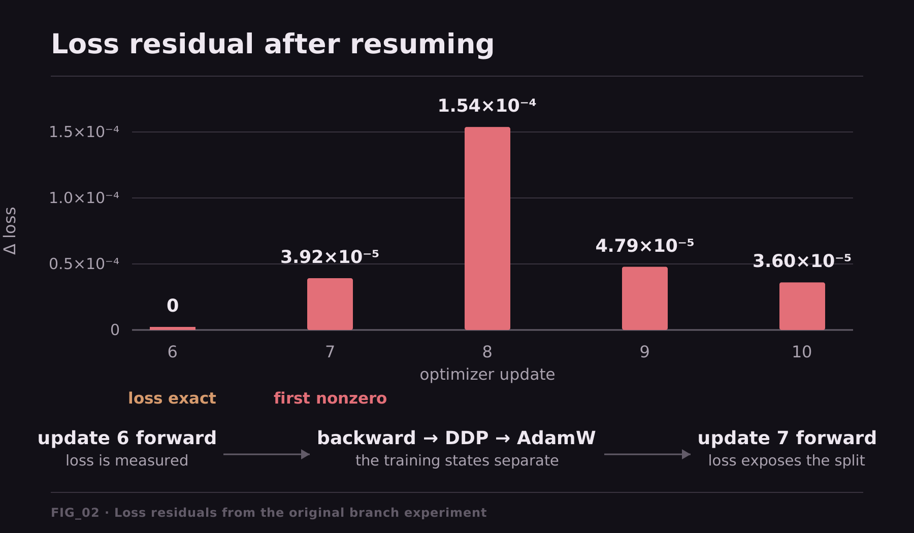
Under deterministic causal convolution and frozen rank-private autotune caches, the original branch experiment produced this loss trajectory:
| Update | Continuous | Resumed | Resumed minus continuous |
|---|---|---|---|
| 6 | 0.8891351451286653 | 0.8891351451286653 | 0 |
| 7 | 0.7142631975696954 | 0.7143024200392002 | 3.92224695048e-5 |
| 8 | 0.7170564289286161 | 0.7172102567508438 | 1.53827822228e-4 |
| 9 | 0.8850533259143935 | 0.8851012246732742 | 4.78987588807e-5 |
| 10 | 0.8002184667904964 | 0.8002545058376878 | 3.60390471914e-5 |
The exact update-6 loss was not comforting. Loss is computed during the forward pass. DDP gradient reduction and the optimizer step happen afterward. A difference introduced during update 6 becomes visible in the scalar loss only when update 7 runs with changed parameters.
Walk backward from the final mismatch
At the end of the failing branch experiment, the embedding mismatch told me only that the trajectories had separated. It did not identify the transition that separated them. I added captures at increasingly earlier boundaries around update 6.
The first pass established that these were exact across continuous and resumed legs:
- scheduled pack indices and stable pack identities
- token IDs, position IDs, supervised targets, padding, and document maps
- model, optimizer, scheduler, trainer, and RNG state immediately before the update
- the normalized forward loss
- the rank-local gradient tensors after the first
no_sync()microbatch - the accumulated rank-local gradient tensors immediately before all-reduce
Then the boundary split:
- immediately after DDP reduction, 261 of 320 full gradient tensors differed on every rank;
- the total pre-clipping L2 norm over all parameter gradients was exactly 2.790245771408081 in both legs;
- clipping preserved the same 261 differing gradient tensors;
- after fused AdamW, 27 model tensors and 513 optimizer tensors differed;
- scheduler and RNG state remained exact.
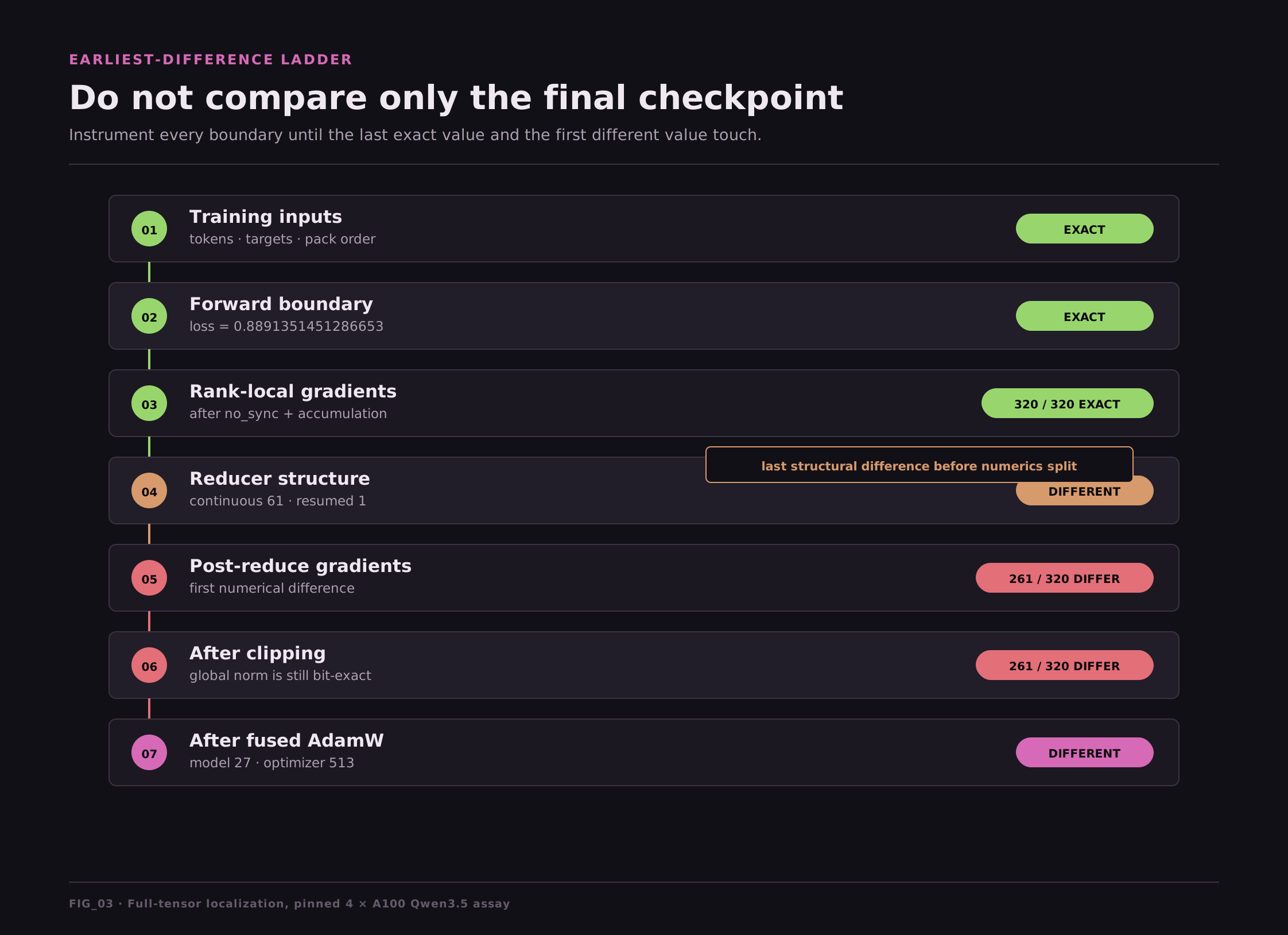
The bit-exact global norm is worth pausing on. A scalar invariant can match even when hundreds of gradient tensors do not. Global norm collapses a high-dimensional object into one value. It is a useful guardrail, not an equality proof.
I now had a precise statement:
The local mathematical backward was exact. The first numerical difference appeared while those exact local gradients were being reduced across ranks.
That localized the difference to the reduction boundary, but it did not explain why the reductions differed. I needed to ask whether both processes had issued the same sequence of reductions over the same groups of elements.
The DDP reducer has an age
Each DDP rank owns a complete model replica, but wrapping that model in DistributedDataParallel also constructs process-local runtime machinery. The relevant object here is PyTorch’s C++ reducer. It installs autograd hooks on the trainable parameters, tracks when their gradients become ready, groups those gradients into flat communication buckets, launches an all-reduce when a bucket is complete, and places the reduced values back into the parameter gradient buffers.
parameter gradient becomes ready
              ↓
autograd hook notifies the reducer
              ↓
the reducer marks one bucket entry ready
              ↓
all entries in that bucket are ready
              ↓
NCCL all-reduces the bucket
              ↓
reduced values return to parameter gradients
The reducer is a runtime object owned by one DDP process, with its own bucket membership, communication sequence, and lifecycle flags. A checkpoint can restore every model and optimizer tensor without restoring this object.
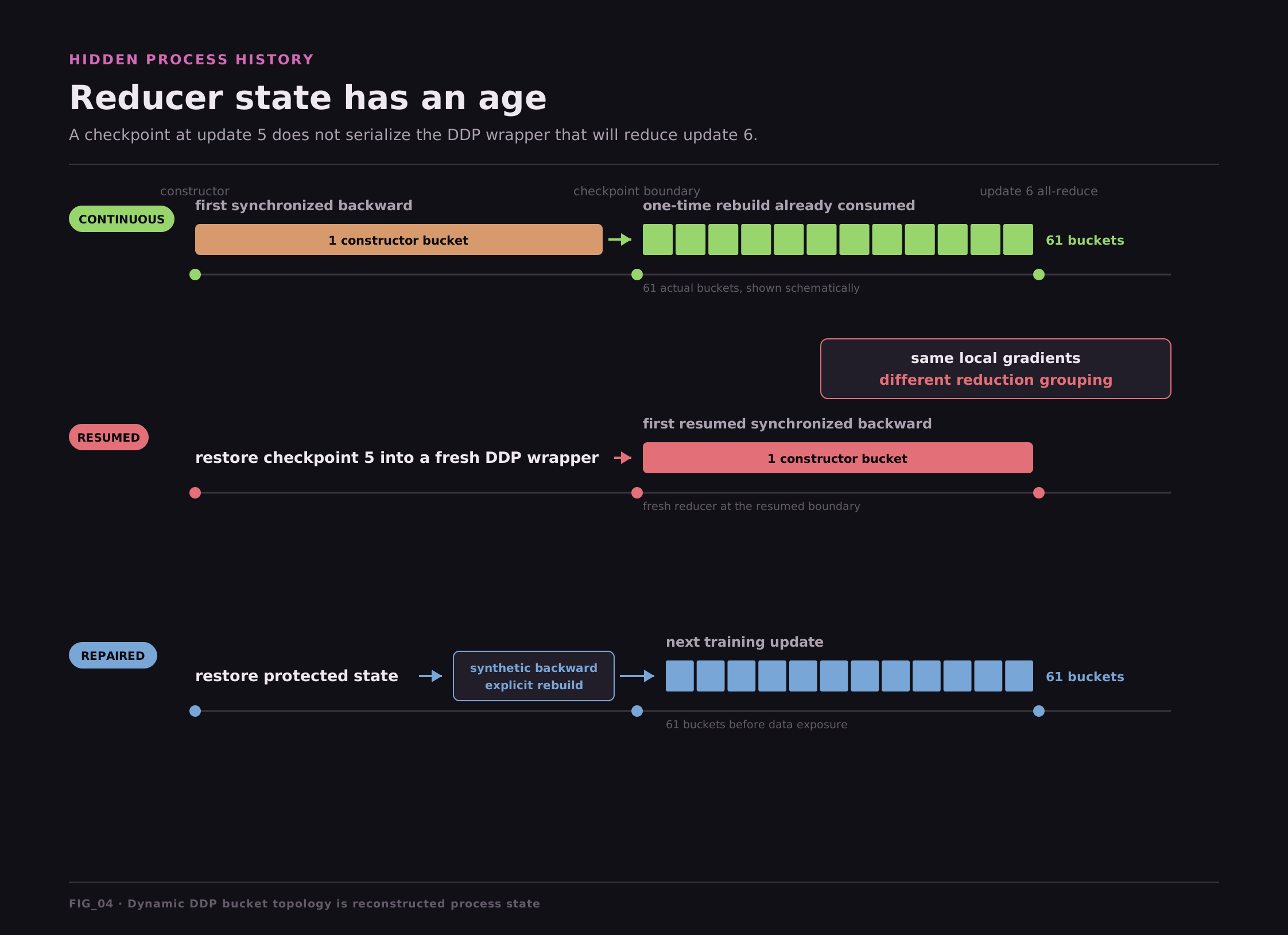
Once the full gradient captures showed exact values immediately before reduction and different values immediately afterward, I recorded the reducer’s structure at that boundary. For every collective, I retained the bucket index, ordered parameter membership, element count, and launch sequence. The continuous process entered update 6 with 61 ordered buckets. The resumed process entered the same update with one bucket containing all 320 trainable parameters. Both layouts covered the same 752,393,024 FP32 elements, but they did not submit the same grouping of those elements to the collective layer.
In my configuration with find_unused_parameters=False, DDP did not begin with its final communication layout. The reducer moved through a short lifecycle:
- A newly constructed DDP wrapper placed all parameters in one initial bucket
- During the first synchronized backward, the reducer observed the order in which parameter gradients became ready
- Before a subsequent forward pass, it used that observed order to rebuild the single bucket into the normal bucket layout
- That rebuilt layout was then reused for the rest of training
Only the second microbatch exercised the reducer. The first update-6 microbatch ran inside no_sync() and accumulated local gradients without communication. The second microbatch performed the synchronized backward. In the fresh resumed process, that backward was the reducer’s first real reduction and therefore still used the constructor bucket.
PyTorch source references. The pinned implementation shows the initial single-bucket construction, the one-time rebuild before a subsequent forward pass, and the C++ reducer’s gradient-ready order and bucket-rebuild state transition.
These are process-local DDP internals rather than ordinary checkpoint state. I would not expect most training frameworks to serialize them, and Open-Instruct did not. When the resumed job constructed a new DDP wrapper, it also constructed a new reducer with a fresh lifecycle. Restoring checkpoint 5 populated the model, optimizer, scheduler, trainer, and RNG state, but it did not populate the reducer’s ready-order history or mark its one-time rebuild as complete.
By update 6, the continuous reducer had already passed through synchronized backwards during updates 1 through 5 and matured into 61 buckets. The resumed reducer had the same model parameters but none of that process history. It was still at its one-bucket constructor state.
Why legal reductions can produce different FP32 values
For real numbers, addition is associative. For floating-point numbers, rounding happens after each operation:
\[ \operatorname{fl}(\operatorname{fl}(a+b)+c) \neq \operatorname{fl}(a+\operatorname{fl}(b+c)) \]Changing a bucket boundary can change how elements are flattened, combined, divided, and copied back. The collective can obey its contract in both runs while the final FP32 bits differ. The relevant question is not “did NCCL return a valid all-reduce?” It is “did both legs submit an equivalent reduction program?”
The full-tensor boundary capture made the causal ordering unusually clean:
| Boundary | Continuous | Resumed | Comparison |
|---|---|---|---|
| Accumulated local gradients | 320 tensors | 320 tensors | all exact |
| Ordered reducer layout | 61 buckets | 1 bucket | different |
| Post-reduction gradients | 320 tensors | 320 tensors | 261 differ |
Reconstructing reducer state before training
Once the mechanism was localized, the intervention followed directly: every newly constructed DDP reducer had to reach the same mature layout before it reduced a real training update.
I call that initialization step a reducer prime. It is a protected, non-optimizing synthetic forward and backward whose only intended persistent effect is to let the reducer observe a complete gradient-ready order and materialize its steady-state bucket layout. It does not prime the model parameters, optimizer, scheduler, or training data.
The policy applied independently whenever a DDP wrapper was constructed. In the continuous leg, I primed that process’s reducer before update 1. In the resumed leg, I restored checkpoint 5 into a different process and then primed that process’s new reducer before update 6. The resumed process did not modify or communicate with the continuous process; each process initialized its own reducer.
I did not serialize the C++ reducer object. That would bind a checkpoint to opaque implementation state and make compatibility harder to reason about. Instead, I reconstructed the relevant state deterministically in every fresh process before it saw a real training pack.
The reducer initialization performed this sequence:
- validate that the wrapper exactly matches the qualified DDP configuration
- snapshot every state category that the prime is forbidden to change
- construct a deterministic synthetic sequence of length 32,768
- select 1,025 causal targets per rank, 4,100 globally
- run a training-mode forward and backward that activates all 24 checkpointed layers
- explicitly call the reducer’s one-time bucket rebuild
- clear all gradients
- restore RNG, module modes, trainer bookkeeping, and loss-audit state
- verify that model tensors, buffers, parameter version counters, optimizer state, scheduler state, trainer state, RNG state, and absent gradients are unchanged
- only then give the process its first real training batch
The model did not materialize vocabulary logits for all 32,768 sequence positions at once. Only 1,025 positions on each rank carried causal targets. At each of those positions, the selected-output loss projected the hidden state through the vocabulary head and computed its cross-entropy contribution.
To bound peak memory, the same loss path used by the actual training run processed those selected positions in three half-open chunks: [0, 512), [512, 1024), and [1024, 1025). The first two chunks contained 512 supervised positions each and the last contained one. Their loss contributions were combined using the trainer’s global-token normalization. In real arithmetic, partitioning the supervised positions this way leaves the objective unchanged:
Floating-point reductions can nevertheless depend on how terms are grouped. The reducer initialization therefore reproduced the actual training run’s chunk boundaries, operation order, dtypes, loss normalization, and backward scaling. It exercised the same numerical path without taking an optimizer step or advancing the scheduler.
A synchronized backward is what gives a fresh reducer the missing history. This code ran once during process initialization, after constructing the DDP wrapper and restoring any checkpoint but before fetching the first real training batch. It was not part of the per-update training loop. The reducer-changing core was small:
# ddp is torch.nn.parallel.DistributedDataParallel(model)
# Each rank executes a deterministic, full-graph synthetic pass.
outputs = ddp(**synthetic_inputs)
loss = compute_the_normal_training_loss(outputs, synthetic_targets)
loss.backward()  # records the order in which gradients become ready

# Materialize the normal bucket layout from the recorded order now,
# before the first real training batch.
rebuilt = bool(ddp.reducer._rebuild_buckets())
if not rebuilt:
    raise RuntimeError("expected the one-time reducer rebuild")
ddp._has_rebuilt_buckets = True

# The synthetic gradients must never reach the optimizer.
ddp.zero_grad(set_to_none=True)
Here, ddp is the model after PyTorch has wrapped it in DistributedDataParallel. The synthetic backward() runs through every trainable parameter, allowing the reducer to observe a complete gradient-ready order. The private _rebuild_buckets() call converts that order into the normal bucket layout, and _has_rebuilt_buckets keeps the Python wrapper’s bookkeeping consistent with the C++ reducer. No optimizer step follows, and the gradients are cleared immediately.
On the expected first call, _rebuild_buckets() returned true: the synchronized backward had recorded the gradient-ready order, and the reducer had not rebuilt yet. A false return meant that the expected lifecycle transition had not occurred. A wrapper that had already rebuilt, an incomplete synthetic backward, or a changed DDP implementation could all cause that outcome. The surrounding initializer handled cleanup on failure and stopped the process before any real training data was consumed.
compute_the_normal_training_loss is the only placeholder in the sketch. It means the selected-output loss, chunking, global-token normalization, and backward scaling described immediately above. The surrounding implementation also snapshotted and restored RNG state, module modes, trainer bookkeeping, and loss-audit state, then verified that the synthetic pass had changed nothing except the reducer lifecycle.
For this experiment, I also recorded the conditions under which I had validated the initialization:
- exact PyTorch
2.9.1+cu129source identity; - a native C++ DDP reducer over an initialized NCCL process group;
- world size 4 or 8;
- dynamic DDP with
find_unused_parameters=False; gradient_as_bucket_view=False;- a 25 MiB bucket cap;
- no communication hooks, delayed reductions, ignored parameters, or DDP mixed-precision mode;
- a wrapper that had not already rebuilt its buckets.
As a reminder, _rebuild_buckets() is a private PyTorch API and should be avoided in production code when possible.
Why static_graph=True was not the repair
It is tempting to interpret “static” as “stable from construction.” That is not what this reducer lifecycle guarantees. In my source-bound control, the static-graph path produced bucket counts [1, 1, 8]. It delayed the rebuild, so it delayed rather than removed the age mismatch.
Likewise, find_unused_parameters=True was not a free switch. It conflicted with the chosen gradient-checkpointed training contract. Resume correctness has to be repaired inside the tested training configuration, not by silently changing the training algorithm.
The causal test: change the layout, keep the local gradients
The next causal experiment repeated the exact update-6 comparison with each process initializing its own reducer as described above. It was designed so that the intervention changed the suspected cause before the training boundary and nothing else.
This was a new paired experiment, not a modification of the earlier continuous process. Its continuous leg used the mature 61-bucket layout from update 1, whereas the original continuous leg had used the constructor layout for its first update and matured afterward. Those two continuous trajectories therefore belonged to different initialization policies and were not compared to each other. Within the new experiment, however, the continuous and resumed legs followed the same policy and could be compared directly.
| Experiment | Continuous buckets | Resumed buckets | Local gradients | Post-reduce gradients | Update boundary |
|---|---|---|---|---|---|
| Baseline: no reducer initialization | 61 | 1 | 320 / 320 exact | 261 / 320 differ | different |
| Intervention: initialize both reducers | 61 | 61 | 320 / 320 exact | 320 / 320 exact | exact |
The negative control had the structural mismatch and the numerical mismatch. The intervention removed the structural mismatch while preserving the local mathematical inputs. The numerical mismatch disappeared at the predicted boundary.
The result supports this causal statement inside the pinned system:
DDP bucket-layout age was necessary for the observed post-reduction divergence once rank-local kernel and autotune differences were controlled.
It does not say that bucket count alone determines every bit. Ordered bucket membership matters, not just the scalar count. My validator compared the complete ordered layout and full gradient tensors.
Confirmation in the full training run
The final confirmation returned to the complete branch geometry. One leg trained continuously from updates 1 through 10, with its reducer initialized before update 1. A fresh four-rank process restored checkpoint 5, initialized its own reducer, and then trained updates 6 through 10.
Every resumed loss was exactly equal:
| Update | Continuous | Resumed | Difference |
|---|---|---|---|
| 6 | 0.8891536212776797 | 0.8891536212776797 | 0 |
| 7 | 0.7142767564822723 | 0.7142767564822723 | 0 |
| 8 | 0.7170606408808914 | 0.7170606408808914 | 0 |
| 9 | 0.8850564095254803 | 0.8850564095254803 | 0 |
| 10 | 0.8001803865937296 | 0.8001803865937296 | 0 |
At update 10, zero-tolerance comparison found:
model tensors             320 compared,   0 nonidentical, max abs difference 0
optimizer tensors         960 compared,   0 nonidentical
optimizer scalars         346 compared,   0 nonidentical
scheduler state                          exact
Python RNG                               exact
NumPy RNG                                exact
CPU Torch RNG                            exact
CUDA RNG, ranks 0 to 3                   exact
deterministic trainer state              exact
ten stable log entries                   exact
The schedule, pack identities, target counts, loss projections, padding and document maps, selected-output audits, gradient audits, and learning-rate projections were also exact.
That is the result I wanted from the beginning. The final equality alone, however, does not explain what happened. The causal evidence comes from the sequence of boundary comparisons and controlled interventions that showed where equality first failed and which runtime state restored it.
What the loss curve did and did not tell me
Loss curves are useful for discovering that trajectories differ. They are weak tools for locating why.
In this case, update 6 had the same loss in both branches because the loss was computed from exact parameters and exact inputs before the differing reduction. The all-reduce and optimizer changed the parameters later in the update. Update 7 was the first scalar observation made from those changed parameters.
That timing is the important limitation. The loss at a given update describes the forward pass before that update’s backward and optimizer step. Once the loss curve diverges, it exposes the consequence of an earlier parameter update rather than the location where the executions first became different.
Scalar summaries compress information in a similar way. At update 6, the total pre-clipping L2 norm over all parameter gradients was exactly 2.790245771408081 on every rank in both legs, while 261 of 320 full gradient tensors differed. The matching norm established only that the reduction to one scalar produced the same value, not that the underlying gradients were identical.
None of this means that a bitwise-different resume is unusable. For ordinary model development, statistical reproducibility may be the right target, and exact equality can be unnecessarily expensive.
Find the first different boundary
The most useful debugging rule from this investigation was to compare the continuous and resumed branches in execution order:
checkpoint bytes exact?
  → live state after restore exact?
    → training inputs exact?
      → forward outputs and loss exact?
        → rank-local gradients exact?
          → accumulated pre-reduce gradients exact?
            → reducer structure exact?
              → post-reduce gradients exact?
                → clipped gradients exact?
                  → optimizer outputs exact?
                    → next forward exact?
The last exact boundary and the first different boundary bracket the cause. In this case, the accumulated gradients were exact before reduction, the reducer structure differed, and the gradients differed immediately after reduction. That sequence narrowed the investigation to the reducer and all-reduce boundary before the bucket-lifecycle mechanism was known.
What should a resume system preserve?
I am not arguing that training frameworks should expose and checkpoint every low-level runtime detail. That would be brittle and, for most training goals, unnecessary. The ideas below are simply the design questions this investigation left me with for cases where exact continuation matters.
There are two defensible strategies for hidden runtime state.
Serialize it
This works when the state has a stable, public, versioned representation. Optimizer moments and scheduler counters belong here. A framework can validate compatibility before loading.
Reconstruct it deterministically
This is often safer for opaque runtime objects. Instead of serializing PyTorch’s private C++ reducer internals, I reconstructed the qualified bucket layout with a protected, non-optimizing prime. Instead of serializing live Triton Python objects, I froze their portable cache records and loaded identical rank-private copies.
The important part is not which strategy wins in the abstract. The resume contract must name the state and prove that the chosen strategy makes both branches equivalent before it can affect the next training update.
A practical state inventory for modern distributed training should at least consider:
| State category | Typical examples | Likely treatment |
|---|---|---|
| Persistent numerical state | parameters, buffers, optimizer moments | serialize and compare exactly |
| Progress state | scheduler, update counters, data cursor | serialize with semantic validation |
| Randomness | Python, NumPy, CPU and device RNG | serialize per process and device |
| Kernel selection | autotune records, algorithm flags | freeze or reconstruct deterministically |
| Communication state | ordered buckets, hooks, collective schedule | reconstruct and validate before exposure |
| Compilation state | graphs, guards, code caches | pin inputs or qualify recompilation |
| Data realization | packing, sharding, worker queues | record identities at the rank boundary |
This inventory is not a demand to hash every file in sight. Validation should sit at boundaries that can change the training result. Once a kernel cache has been frozen and its effective records verified, repeatedly rehashing an unrelated tree does not make the next optimizer update more trustworthy.
Framework-level implications
Training frameworks often advertise checkpoint completeness in terms of objects they own: model, optimizer, scheduler, dataloader, and RNG. The missing states in this investigation lived below or beside that abstraction.
Open-Instruct owned the training loop and selected-output loss path. Transformers and Accelerate helped construct and drive distributed training. PyTorch owned the DDP reducer lifecycle. causal-conv1d owned one backward algorithm. FLA and Triton owned autotuning and caching. NCCL executed collectives over buckets defined elsewhere.
No single layer had a complete view of resume equivalence.
That suggests a better framework contract:
- enumerate all stateful runtime components on the update path
- let each component declare whether its relevant state is serialized, deterministic from configuration, or process-history dependent
- expose public initialization hooks for history-dependent state
- run those hooks before data workers or the trainer consume real training examples
- validate the first resumed update at meaningful boundaries in a qualification test
The DDP repair in this post uses a private API because PyTorch did not expose the exact public lifecycle operation I needed. A public “materialize the steady-state reducer layout without an optimizer step” contract would be easier for training frameworks to support safely.
Limitations
The strongest conclusion is also the narrowest one.
- The exact full-run confirmation covers Qwen3.5-0.8B, one node, four A100s, pure dynamic DDP, gradient accumulation two, and the pinned software stack.
- It does not establish exact resume for FSDP, tensor parallelism, context parallelism, HSDP, multiple nodes, or another collective backend.
- It does not establish that every hidden process state must be controlled for statistical reproducibility.
- The reducer intervention depends on private PyTorch APIs and must be requalified for any source change.
- The frozen Triton-cache experiment initially used sampled fingerprints for most gradients. The later reducer experiments rely on full gradient tensors at the relevant boundary.
- Ten updates are enough to prove or refute exact continuation in this branch, but not to characterize the long-horizon statistical impact of the original drift.
There is also a broader experimental caveat. Exact equality is easier to falsify than to generalize. One unequal bit proves that two executions are not bitwise identical. Ten equal updates in one qualified system do not prove that every future model and runtime will resume exactly.
The lesson
The first mismatch at the distributed boundary did not come from NCCL producing different results for the same collective schedule. The rank-local gradients were exact, but DDP submitted them as 61 ordered buckets in the continuous process and one bucket in the resumed process. NCCL therefore executed different valid collective sequences over differently sized FP32 buffers, and those reductions produced different rounded values.
Checkpointing and resumption are two stages of the same recovery workflow. Recovering from an interruption is one of the main reasons to save a checkpoint, but the checkpoint file alone does not define the behavior of the new process:
- checkpointing captures the durable state at a training boundary
- resumption restores that state and reconstructs the process-local runtime machinery needed for the next update
Once training stacks include fused kernels, autotuners, compilation, gradient accumulation, and distributed reducers, part of the executed algorithm can depend on process history. If that history is neither serialized nor deterministically reconstructed, the checkpoint can load correctly while the next update already differs from uninterrupted execution.
Source anchors
Comments
Comments will appear here once Giscus is configured.