Position Information in Transformer-Based Models: Exploring the main Methods and Approaches

This post will only focus on some position encoding, namely, sinusoidal, T5 bias, ALiBi and Rotary. It’ll also discuss no position encoding (NoPE) and FIRE (functional interpolation of relative position encoding) This choice was made because the first methods are the most present in comparative benchmarks while for NoPE and FIRE, I found the ideas and the maths behind them interesting so I wanted to talk about them as well. These methods cover a good range of the ideas used in position encodings so understanding them gives insight into many other position encoding methods that were developed at the same time.

Introduction: Position Encoding

Position encoding in sequence to sequence settings is a way to encode the position of each token in a sequence. Some model architectures implicitly encode that information, like RNNs and CNNs (more about that here and here), while others don’t, like purely attention-based transformer architectures. But, there’s a catch with purely attention-based transformer architectures. Encoder-only Transformers, without positional encoding, are equivalent to a bag of words model (see here) but it is not the case in transformer architectures that use causal self-attention like the decoder-only models, which is proved in The Impact of Positional Encoding on Length Generalization in Transformers and which we discuss in detail in our sixth section about NoPE.

Do we need Position Encoding or not?

Let’s first see what is the idea behind encoding position. The attention computation of, say element $i$ in the input sequence, involves the dot-product between the query of the $i$-th element and the keys of all other elements $j$ (in causal self-attention $j \leq i$) , $$. The result from this dot-product doesn’t contain any information on the positions of $i$ and $j$ in the sequence. It only contains information about the lengths of the vectors and the angle between them (we’ll see later that RoPE uses this idea). Though its input are sequences, the attention operation can be seen as an operation on sets, thus its result does not take into account any relation (thus any ordering) you might define on your set.

But intuitively, we should not weigh the dot-product between $i$ and $j_{1}$ when $i - j_{1} \geq 100$ the same as the dot-product between $i$ and $j_{2}$ when $i - j_{2} \leq 5$. Otherwise, what we’d obtain is the same thing as a bag of words.
That’s when the idea of position encoding intervenes, it’s an inductive bias we inject in the network to help it learn better and build better representations by taking into account the positions of the tokens.

The paper The Impact of Positional Encoding on Length Generalization in Transformers demonstrates that position encoding in causal attention is not useful though, because the network will learn some kind of internal position encoding by itself.

Though when discusssing position encoding, we should distinguish between two aspects, the training of the network on sequences with the same fixed length and its generalization capability during inference to sequences with lengths greater than the one the network was trained on, what we generally see in the papers is a focus on the generalization capability that the method offers because the training is a given. There’s no discussion about generalization but if the model can’t even be trained.

Properties We Want in Position Encoding

There are some properties that we want in the position encoding methods that we will elaborate. The main properties that I could gather by reading the papers are:

• Memory: how much memory does the method add when training
• Time: how much slower the training becomes when using the method
• Length generalization: the generalization capability to sequence lengths unseen during training that the method offers

Some papers do include the following property as well, but I’m not sure of it:

• Long-term decay: this property pertains to relative positional encodings only where we encode the distance between two positions. So, it makes sense that our method should lead to a stronger relationship between tokens closer to each other compared to tokens that are far from each other

I’m unsure of it because T5’s position encoding method doesn’t verify it and it seems to work well. In FIRE, the PEs are learned as well so I doubt they verify some kind of long-term decay but I don’t have access to networks trained with this method to verify it.
The argument for having the long-term decay property is quite self-explanatory, and it’s kind of an inductive bias that we’re introducing. And we can can also make an argument against it and say that we’d like to have different patterns, preferably learned by the network. We’ll discuss that in the T5’s section.

Note: Although we’re studying the position encoding methods in the context of auto-regressive models, the same principle can be used in other contexts, for example in an encoder. The absolute position encodings are quite straight-forward in their adaptation to the general case, and for the relative position encodings we just have to replace the causal part of the mask with a symmetrical version of the biases part with respect to the diagonal.

Mathematical Framework

In this section we establish the mathematical framework to provide a common ground in exploring and discussing the position encoding methods. This framework is the same as the one used in RoFormer: Enhanced Transformer with Rotary Position Embedding, and we’re going to use it for the other methods as well. Unless explicitly mentioned, we’re going to follow exactly the framework in the paper.

Let $\mathbb{S}_{N} = \{w_{i}\}_{i=1}^{N}$ be a sequence of $N$ input tokens with $w_{i}$ being the $i^{th}$ element. The corresponding word embedding of $\mathbb{S}_{N}$ is denoted as $\mathbb{E}_{N} = \{\boldsymbol{x_{i}}\}_{i=1}^{N}$, where $\boldsymbol{x_{i}}\in \mathbb{R}^{d}$ is the $d$-dimensional word embedding vector of token $w_{i}$ without position information.

At this stage, we’re ready to apply some transformation on $\mathbb{E}_{N}$ either at the bottom level of the architecture, meaning before the first multi-head attention sub-layer, e.g. add to $\mathbb{E}_{N}$ sinusoidal position encoding, or at the level of the attention computation, e.g. ALiBi.

In order to keep a general framework we can write the queries, keys and values as functions of $\mathbb{E}_{N}$ and of the positions where the functions include the linear projection to obtain the queries, keys and values, as well as a mechanism to include the position encoding, which leads to the first set of equations as described by the authors:

Where $\boldsymbol{q_{m}}$, $\boldsymbol{k_{n}}$ and $\boldsymbol{v_{n}}$ incorporate the $m^{th}$ and $n^{th}$ positions through $f_{q}$, $f_{k}$ and $f_{v}$ respectively.

The attention weights are computed as follows:

Where $\boldsymbol{o_{m}}$ are the outputs of the attention-mechanism, the weighted sum of attention weights of the values.

In the following sections, we’ll use $L$ to denote the maximum sequence length that a model is trained on.

Let’s now discus, under this framework, some absolute position encoding methods.

Absolute Position Encoding

Absolute Position Encoding (APE) methods use a set of encoding vectors $\{\boldsymbol{p_{i}}\}_{i}$, of dimension $d$, at the token embedding level. In contrast, Relative Position Encoding (RPE) repeat the position encoding at each attention layer.

We’re going to discuss two main methods used in the APE setting: learned position encodings, and the non-parametric method relying on sinusoidal functions. In both cases, the equation $(1)$ becomes

Learned Position Encoding

These position encodings are learned as parameters of the model. So the model learns exactly $L$ vectors $\boldsymbol{p_{i}}$ of dimension $d$, so we add $L\times d$ parameters to the model. Some models that use this setting are BERT and GPT.

This way of encoding positions is not generalizable at all since we have a fixed set of position encoding vectors. One can use a similar method as in BERT where they pre-trained the model 90% of the steps on sequence lengths of size 128 then on sequence lengths of size 512 but it’s definitely not a flexible method since that will require extending the pre-training on different sequence lengths each time one wants to extend and it’s not optimal for downstream tasks that require way larger sequence lengths.

Here’s an example of adding learnable position encoding to your model. I’m going with nn.Parameter instead of nn.Embedding but both work. You should fill in your own model’s logic in the following example

class Model(nn.Module):
    def __init__(self, config):
        super().__init__()
        ...
        self.tok_emb = nn.Embedding(config.vocab_size, config.n_embd)
        self.pos_emb = nn.Parameter(torch.zeros(1, config.context_size, config.n_embd))
        self.dropout = nn.Dropout(0.1)
        ...

    def forward(self, sequence):
        _, T = sequence.size()
        token_embeddings = self.tok_emb(sequence)
        position_embeddings = self.pos_emb[:, :T, :]
        x = self.dropout(token_embeddings + position_embeddings)
        ...

Non-Parametric Sinusoidal Position Encoding

These were introduced in the original transformer paper, Attention Is All You Need. The authors did experiment with the learned position encodings but found that both lead to the same performance as they say:

We also experimented with using learned positional embeddings [9] instead, and found that the two versions produced nearly identical results (see Table 3 row (E)). We chose the sinusoidal version because it may allow the model to extrapolate to sequence lengths longer than the ones encountered during training.

Reframing their equations in our framework we get these vectors $\boldsymbol{p_{i}}$:

So, for each position $i$, the value for each pair position in its positional encoding vector is computed using the $sin$ equation, and the value for each impair position in the encoding vector is computed using $cos$ equation.

The following figure shows how the values for each of the $6$ first dimensions change across the positions in a sequence. We also show the values of the first 5 positions which are the values are the top of the red dotted lines. The plots are for $d=512$.

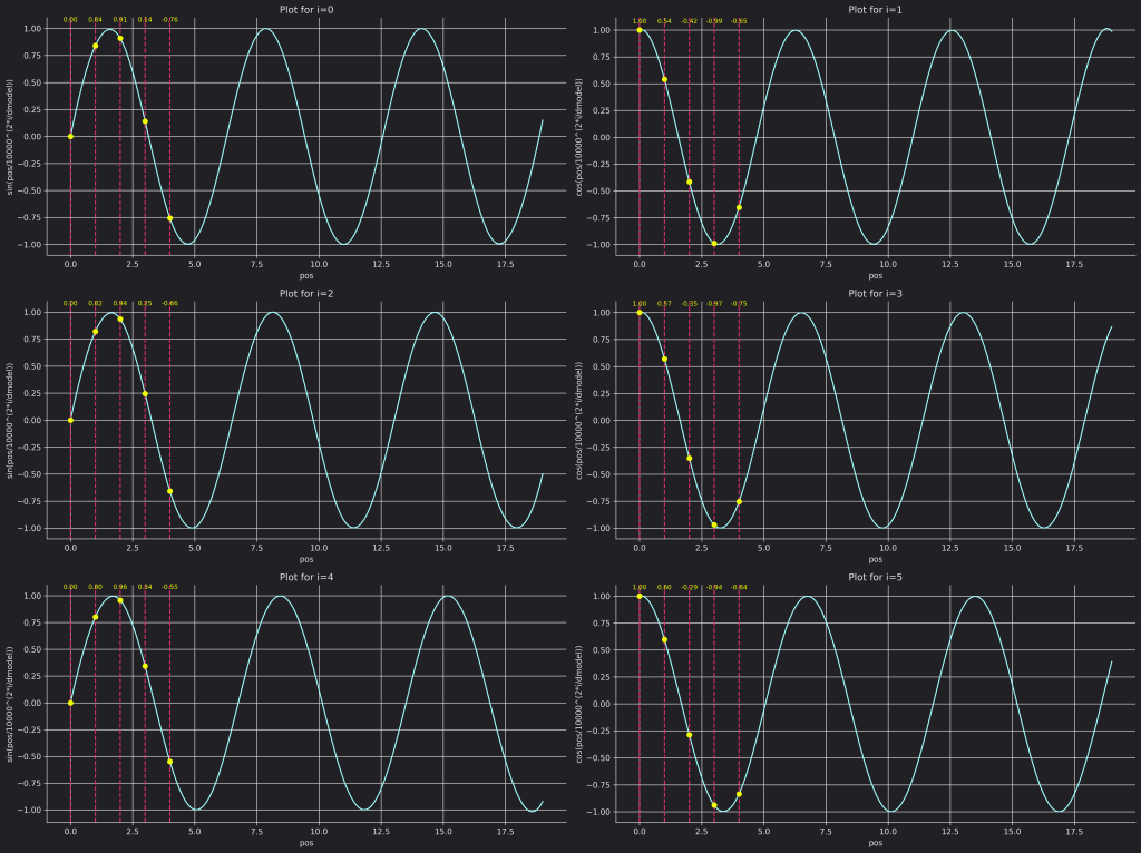
Though the equation allows to encode the absolute position for a fairly large number of tokens compared to what the model is generally trained on, the experiments show that this method doesn’t allow the model to generalize at all. My guess is that this is like the famous extrapolation example where we train a model to learn a sinusoidal function on [0, 1] but then it fails to generalize outside of that segment. So for example if we have trained our transformer on sequences of length $1024$, it learns some kind of association between a position and its PE vectors (I’m not totally sure about that, it is just my guess), but then, when we’ll feed it token $1234$ during inference and add to it its PE vector, it is not capable to extrapolate the association it learned to that case.

Here’s a Pytorch code for how one can compute them

def compute_positional_encoding(sequence_size, d_model):
  positional_encoding = torch.zeros((sequence_size, d_model))
  positions = torch.arange(sequence_size)
  indices = torch.arange(d_model // 2)
  
  positional_encoding[:, ::2] = torch.sin(positions[:, None] / (10000 ** (2 * indices / d_model)))
  positional_encoding[:, 1::2] = torch.cos(positions[:, None] / (10000 ** (2 * indices / d_model)))
  return positional_encoding

You can either compute the whole set of position encoding for sequence_size = context_size, your maximum sequence length for which you’re training the model for and cache them. Or you can compute them for your batch’s maximum sequence length each time. There are certainly many optimized ways to do this, but this is just for learning.

Relative Position Encoding

Relative Position Encoding methods try to encode the relative difference in positions between elements into the attention computation. One way to do that is to add some kind of bias to the key-query dot-product (i.e. to the logit used to compute the attention weights). The following methods use this same approach but in a different way. I’m covering them in their order of appearance.

Here we’re going to focus on the matrix $B$ in the following:

You can see it as adding $b_{m,n}$ in the computation of $a_{m, n}$ in equation $(2)$.

So the following methods agree on the approach but not on what $B$ is.

This is like a weighting scheme of the attention weights because now with the softmax instead of having $\frac{e^{q_{i}k_{j}}}{\sum_{r,s}^{}{e^{q_{r}k_{s}}}}$ we’re going to have:

The figure below shows some random attention weights for $i=5$, some kind of $b_{i,j}$ for $j \leq i$ and how it affects the final attention weights:

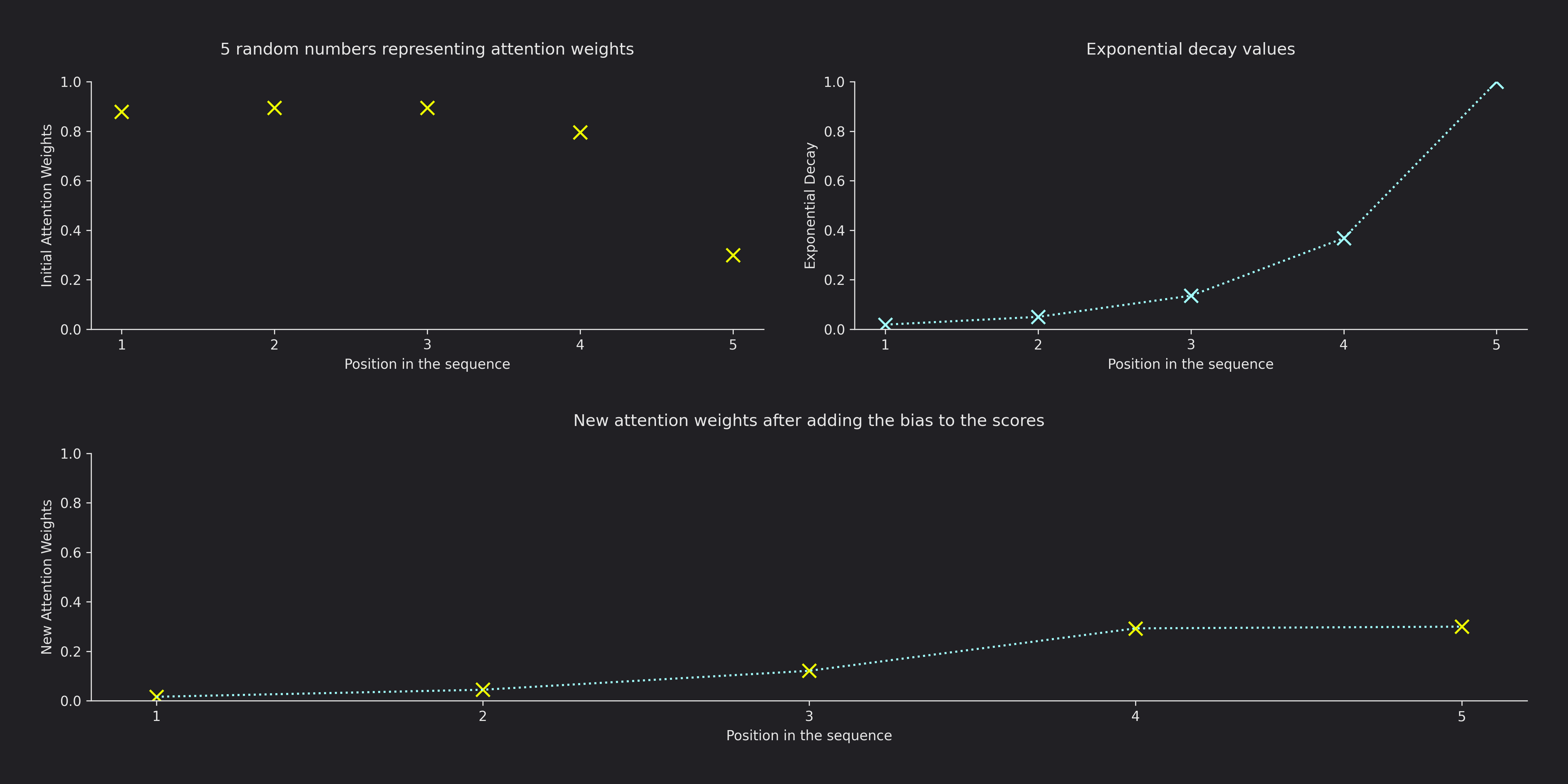
(The figure above is show what happens with ALiBi if $m=1$)

T5’s position encoding method

Paper: Exploring the Limits of Transfer Learning with a Unified Text-to-Text Transformer

Here, $B$ is of shape $(s, num\_heads)$ where $s$ is some number. In [T5’s paper,](http://Exploring the Limits of Transfer Learning with a Unified Text-to-Text Transformer) it is 32. So it’s not exactly what we would add to the query-key dot product, but it’s a lookup table that we’ll use to build the biases used in the scaled dot product.

You can run the following code to check it out:

from transformers import T5Tokenizer, T5ForConditionalGeneration

model_name = "t5-large"
tokenizer = T5Tokenizer.from_pretrained(model_name)
model = T5ForConditionalGeneration.from_pretrained(model_name)

relative_position_bias = model.encoder.block[0].layer[0].SelfAttention.relative_attention_bias.weight
print(relative_position_bias.size())

In the $T5$’s case, $num\_heads=16$, so $B$ is of shape $(32,16)$.

First, we see that its dimensions are way smaller than what typically the query-key dot product yields. So we don’t really add $B$ to that, but $B$ here acts more as a lookup table where we’ll look for the values that we’ll be adding to the query-key dot product.

So for each head, we have 32 scalars that we’re going to be using across all layers. So the heads in the same position share the same vector across all layers. Sharing this across layers was done for efficiency purposes, and there is no reason behind sharing the same vector across all different heads that’s why it’s not done. I think it’s even better to have this being different from head to head.

So let’s say we’re at head $m$ and we have computed the scaled dot product between $q_{i}$ and $k_{j}$. We’re going to look at the $B$ table, get the vector $B(.,m)$ and then we’re going to add a scalar to that dot product according to the following equation (from the official implementation):

Here I used $B_{i,j}$ just for convenience and clarity but what we mean is the relative difference between $i$ and $j$. We’re only looking at one row of the lookup table and we’re indexing by $i-j$ (where $i>j$). $N$ is the number of buckets, $32$ in our case, and $d$ the offset, $128$ in our case, and $b_{.}$ are the learned values of the lookup table. (We assume $N$ is even in the general equation)

Let’s see what the $B$ lookup table looks like:

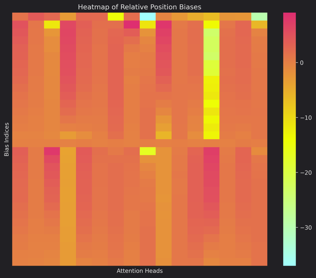
As you can see, there is no real pattern between the different heads’ biases and we don’t have this long-term decay property. As we have seen before (here for example), each heads learns a set of unique representations for some kind of tasks and so I think it is better to not have the same pattern of position encoding biases so that each head learns the bias pattern that works best with the representations it is learning for the kind of tasks it is “solving”.
Also, the fact that there are both positive and negative biases, that are learned, allows some cool choices like increasing the importance of some positions while reducing the importance of others. Though we can have the same with just negative (learned) biases by not increasing the importance of some positions while reducing way more the importance of others, maybe the capability of doing like in the first case helps with convergence and stability of training. (These are just my thoughts)

Attention with Linear Biases (ALiBi)

Paper: Train Short, Test Long: Attention with Linear Biases Enables Input Length Extrapolation

ALiBi is similar to T5’s relative bias but the key differences are:

• ALiBi are not a trainable set of biases. They’re fixed beforehand.
• ALiBi grows indefinitely with the distance between the query position and the key position. In contrast, T5’s relative bias stays the same after the $128$ offset.
• ALiBi’s biases verify the long-term decay property.

So what is ALiBi? The following figure from the paper gives the idea of ALiBi:

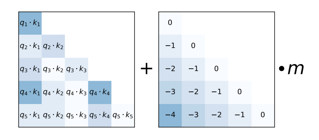
So as one can see, they add scalar biases to the attention score (the query-key dot product). The figure shows the case of causal attention where there’s a mask ensuring there’s no lookahead.

The scalar $m$ depends on the head. It’s a bit like the idea of T5 where each head learns its own set of biases, here each head has its own scalar $m$ and it is the same for all heads of the same position across the layers of the network. The equation for each head is given by $m = 2^{\frac{-8}{n}}$ where $n$ is the number of heads.

I don’t really like how the slope is fixed per head, I’d prefer if each head learned its own slope. But the authors say that it didn’t really impact the results that much. I don’t know if it’s because all the heads have the same kind of bias, the recency bias (the bias grows linearly with the distance between the query and key tokens, which creates a preference toward recent tokens), that learning the slope doesn’t matter that much or not.

The plot below shows at the left show $f(j) = - (i - j) * m$ for a fixed $i=50$ (consider it is the position we’re computing the attention for at the moment). And at the right we show how the attention weights will be changed.

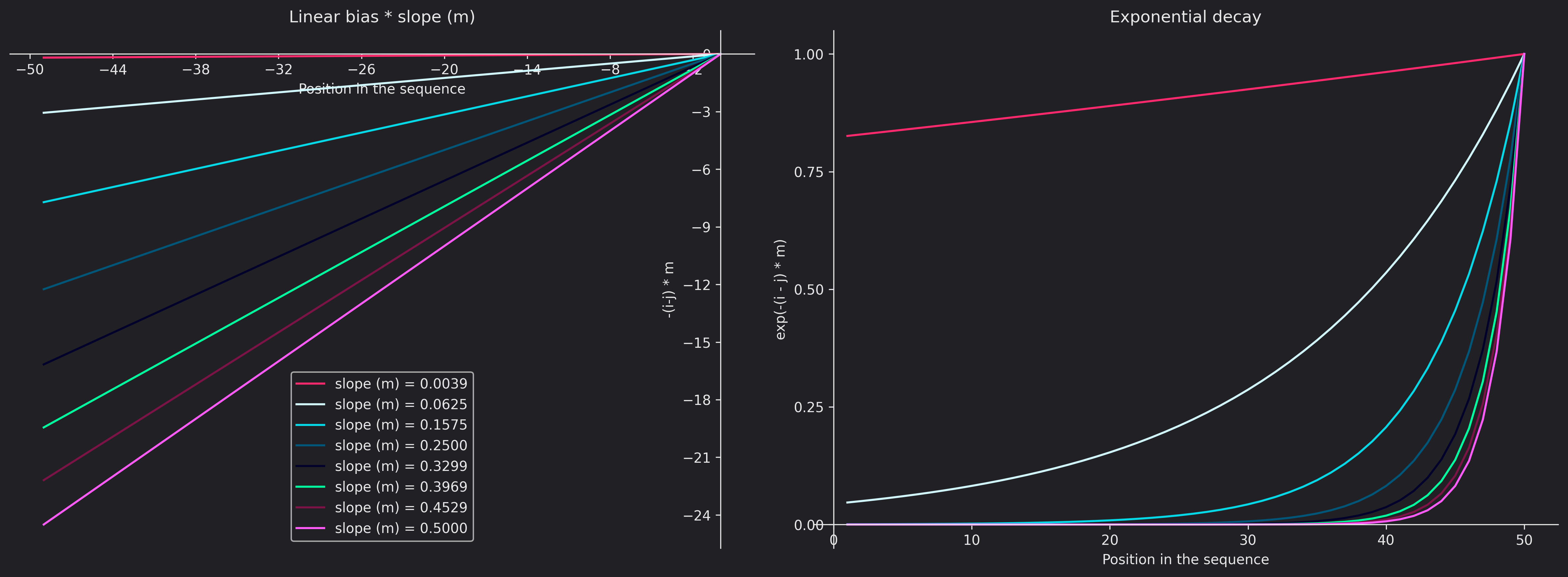
So the more heads we have, the lower the slope $m$ tends to, which makes the “reweighting” of the attention weights behave like a linear plot.

We also notice that for the first few heads we have an effect of “nullification” of many positions starting from a certain offset. In the curve above all the positions from $1$ to $15$ will nearly not participate in the final result of the attention for position $50$ in the first $6$ heads. But these far away positions still contribute in the attention computation in the heads $7$ and $8$, and they contribute more in the head $8$ then head $7$. (Obviously, we are not taking into account here the attention weight itself, but how we’re “reweighting” it with ALiBi, a head can learn some pattern that doesn’t look at far positions at all)

Functional Interpolation for Relative positions Encoding (FIRE)

Paper: Functional Interpolation for Relative Positions Improves Long Context Transformers

It was accepted at ICLR this year (2024): https://openreview.net/forum?id=rR03qFesqk&r

There are many ideas in the FIRE paper, but the main one is taking a functional approach for learning the relative position biases. Instead of hard coding these like in ALiBi or “hard coding” the function that gives the RPE like in T5 (the function is pre-established while the values of the lookup table are learned), the idea of FIRE is to learn that function itself.

So now, $B(i,j) = f_{\theta}(i, j)$ where $\theta$ are the learnable parameters and $f_{\theta}$ maps input positions to relative position biases.

The authors present FIRE and FIRE-S. The latter uses “weight sharing”, which is also used by T5’s RPE and ALiBi, it’s where we have different biases for different heads, but these biases are the same across the layers.

As the authors say “A functional approach to learn the biases allows the model to adapt to the given task instead of always having the same inductive bias”. This way each head, at each layer (in FIRE), will learn the RPE that are the most appropriate to the task the head is learning.

In particular they use an MLP, with two hidden layers and $32$ neurons with ReLU activation function in the hidden layers and no activation function at the output level, to learn these biases. They also prove that this can represent many different RPE techniques like T5, ALiBi etc. The proofs are constructive and use either a two hidden layers or one hidden layer (basically a linear mapping) MLP so we don’t require an arbitrary wide or deep neural network to prove that the FIRE method does represent these other RPE techniques. They also focus on additive RPE techniques and not multiplicative ones like RoPE. Their construction is also parameter efficient, meaning that they represent the same encodings in the same number of parameters up to a constant factor.

Let’s delve into the equation! The general one would be:

$B(i,j)= f_{\theta}(i-j)$ where $f_{\theta}(x) = \boldsymbol{v}_{3}^{T}\boldsymbol{\sigma}(\boldsymbol{V}_{2}\boldsymbol{\sigma}(\boldsymbol{v}_{1}x + \boldsymbol{b}_{1}) + \boldsymbol{b}_{2}) + \boldsymbol{b}_{3}$ and $\theta = \{ \boldsymbol{v}_{1}, \boldsymbol{b}_{1}, \boldsymbol{V}_{2}, \boldsymbol{b}_{2}, \boldsymbol{v}_{3}, \boldsymbol{b}_{3} \}$, $\boldsymbol{v}_{1}, \boldsymbol{b}_{1} \in \mathbb{R}^{32, 1}$, $\boldsymbol{V}_{2} \in \mathbb{R}^{32, 32}$, $\boldsymbol{b}_{2} \in \mathbb{R}^{32, 1}$, $\boldsymbol{v}_{3} \in \mathbb{R}^{32, 1}$ and $\boldsymbol{b}_{3} \in \mathbb{R}$. $\sigma$ is the ReLU activation function.

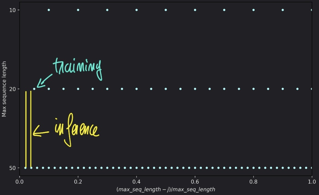
Doing so directly leads to generalization issues. Since the MLP only sees relative distances that are available in the training set, its generalization capability is hurt from that, and so the authors propose Progressive Interpolation to address this challenge; they normalize the query-key relative distance by the query’s position (remember we’re in an auto-regressive context and we’re computing causal self-attention). So the input of the MLP is always in $[0, 1]$. And this is great because as we increase the sequence length, the distance between two different $\frac{i-j}{i}$ decreases (if we were to draw $\frac{i-j}{i}$ for two different values of $i$, for example $i_{1} < i_{2}$, we’ll notice that we’re populating $[0, 1]$ more densely), so this means when we’re using higher sequence lengths during inference, we’ll have more points that fall inside the “buckets” we saw during training and the MLP will be able to extrapolate well to them (this is my interpretation of the authors comment “with increasingly longer sequence lengths, the positional inputs will form progressively finer grids, interpolating the positional encoding function on [0, 1]. Hence, this technique aligns inference domain with training domain for any sequence lengths, leading to better length generalization”). The figure below shows this better, imagine you train on $max\_seq\_length=50$ and then at inference you see a $seq\_length$ of $100$. When computing that normalized relative position, you see that the inference points fall into buckets defined by points see during training, which allows better extrapolation.

So the equation becomes:

$B(i,j)= f_{\theta}(\frac{i-j}{i})$

The authors add two additional transformations:

Amplifying the differences among local positions: With this transformation the equation becomes $B(i,j)= f_{\theta}(\frac{\psi(i-j)}{\psi(i)})$ where $\psi : x \mapsto log(cx + 1)$ where $c > 0$ and is learnable.

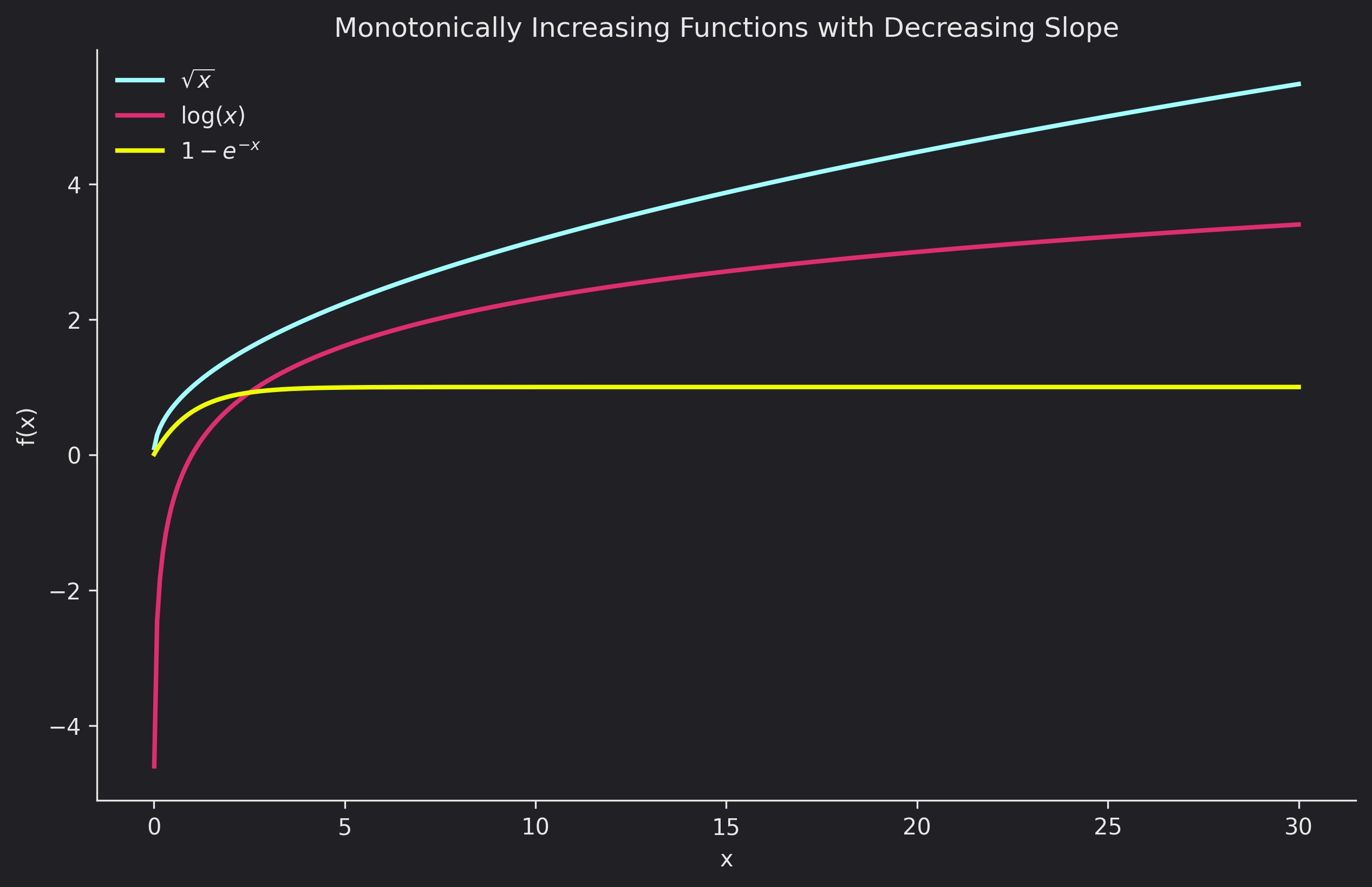
The idea behind this transformation is that the relative position between nearby tokens is more important than with tokens far away from each other. And one way to emphasize that is to use a monotonically increasing function $\psi : \mathbb{N} \to \mathbb{R}_{+}$ with a decreasing slope to the relative distance. This type of function is more sensitive to change at the lowest values since the slope is decreasing, that way our model can capture more fine grained differences with smaller relative positions (i.e. closer tokens). The fact that this helps allocate more modeling capacity can be allocated to learn RPE for local positions stems more from an intuition standpoint I think. Since we have more change between smaller relative position values (in input), the model will focus on learning better biases / encodings (output) for these since there is higher variance in them.

Below are some other functions that have the same property as $\psi$:

The second transformation is: Thresholding the normalizer for better short sequence modeling. The (final) equation is $b_{FIRE}(i,j) = f_{\theta}(\frac{\psi(i-j)}{\psi(max\{L, i\})})$ where $L > 0$ is a learnable.

The authors have noticed during their experiments a slight performance degradation on short sequences and they hypothesized that it’s due to how the normalization affects the RPE in short sequences, compared to longer sequences. Since the relative difference is the most important information to the MLP, we would like to preserve that but in short sequences the denominator is small and we don’t get fine grained normalized relative differences but only rough ones that are fed to the MLP. Thus the idea of using that threshold that is applied to all short sequences.

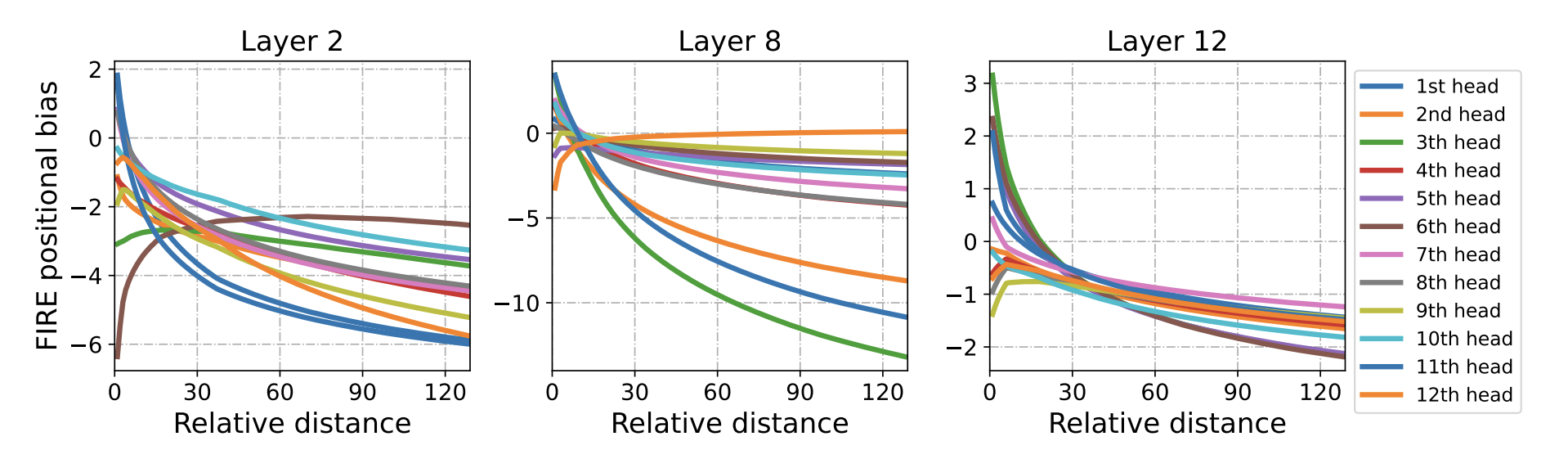
The authors provide us with a visualization of the learned FIRE position biases for the 128th query position (so $i=128)$ with key positions between 1 and 128 (so $j \in [1, 128]$). The authors mention the local and anti-local patterns. I think it’s how the closer positions have these sharp changes in the bias values while it’s more stable towards the far positions.

Both: Rotary Position Embedding (RoPE)

Paper: RoFormer: Enhanced Transformer with Rotary Position Embedding

RoPE is not really either an absolute position encoding or relative position encoding only method but encodes both the absolute position and relative position.

We’ll go over the proof quickly and in a very high-level, just saying what the authors did, so that I can introduce RoPE. Then we’ll see the geometric intuition of it. I feel like the geometry becomes more clear when we have a clear picture of how they constructed the rotary matrix.

For the proof itself, I encourage everyone to read their paper, it’s simple and elegant and I like how they construct their position encoding mathematically. I feel like I saw something similar to this construction in some exercise when studying sesquilinear forms at university, or in quantum mechanics, so it’s pretty cool to see it modified to construct a position encoding method in transformers.

The authors do their construction in 2D but it can be generalized easily, as they say themselves. One can also just plug in the general solution into the attention equation to see that it works as well and is a valid solution.
Their idea starts like this, how can we make the query-dot product $q_{m}^{T}k_{n}$ contain the relative difference in positions between $m$ and $n$. Translating that into math gives: $ = g(x_{m}, x_{n}, m-n)$.

Writing $q_{m} = f_{q}(x_{m}, m)$ and $k_{n} = f_{k}(x_{n}, n)$ in their complex forms as $f_{q}(x_{m}, m)=R_{q}(x_{m}, m)e^{i \Theta _{q}(x_{m},m)}$, $f_{k}(x_{n}, n)=R_{k}(x_{n}, n)e^{i \Theta _{k}(x_{n},n)}$ as well as $g$ as $g(x_{m}, x_{n}, m-n)=R_{g}(x_{m}, x_{n}, m-n)e^{i \Theta _{g}(x_{m}, x_{n}, m-n)}$ and applying some properties of complex vectors and using the fact that these equations hold for all positions the authors find that (well, it’s one of the solutions to be precise) $R_{q}, R_{k}$ and $R_{g}$ are independent of the position. So we can rewrite them as $R_{q}(x_{.}), R_{k}(x_{.})$ and $R_{g}(x_{.}, x_{})$. They even find that $R_{q}, R_{k}$ are the norms of their respective vectors, so $||q||, ||k||$ while $R_{g}$ is the product of both norms $||q||.||k||$, which makes sense knowing how we’re deriving this from the dot-product.

Meanwhile the find that the angular functions do not depend on where they come from, whether the queries or the keys, so they set them to be the same function $\Theta_{f} := \Theta_{q} = \Theta_{k}$. They also find that $\Theta_{f}(x_{i},j)$ can be decomposed as a function of $x_{i}$ and the position $j$ (so the vector and its position are decoupled in this function) and that the function that depends on the position only is an arithmetic progression, so we can rewrite $\Theta_{f}(x_{i},j)$ as $\theta_{i} + m\theta + \gamma$.

Plugging that into our previous equations for $f_{q}$, and $f_{k}$, as well as setting $\gamma = 0$ and using another trick on how the equations are valid for all positions, they find that:

You can see how with these equations the dot product encodes the relative position while the queries and keys contain information about the absolute position.

The general equation is:

Where $\boldsymbol{R}_{\Theta, m}^{d}$, named the rotary matrix, is:

$\Theta$ is pre-defined; $\Theta = \{ \theta_{i} = 10000^{-2(i-1)/d}, i\in [1,2,...,d/2] \}$

You can see how if you want to construct it yourself you should go back to the case of 2D. It’s like some kind of dynamic programming where the solution of a sub-problem helps build the solution of the general problem.

As you can see with this general equation, RoPE works with even embedding dimensions. Since most architectures use an even embedding dimension and since in general they choose powers of $2$ for efficiency of the kernel operations, this isn’t really a constraint.

And the query-key dot-product can now be written as: $q_{m}^{T}k_{n} = \boldsymbol{x}_{m}^{T}\boldsymbol{W}_{q}\boldsymbol{R}_{\Theta, n-m}^{d}x_{n}$

The authors add that:

$\boldsymbol{R}_{\Theta}^{d}$ is an orthogonal matrix, which ensures stability during the process of encoding position information.

I am not totally sure of what the authors imply by “ensuring stability during the process of encoding position information”, but my interpretation is that since $\boldsymbol{R}_{\Theta}^{d}$ is an orthogonal matrix, when we use it to encode information, so the different vectors we gain by doing $\boldsymbol{R}_{\Theta, m}^{d}\boldsymbol{W}_{q,k}x_{m}$ are still in the “same” space. Not really the same space but since this operation is isometric, it preserves the structure and the geometry of the initial space, so we’re not introducing some kind of distortion which would cause information loss. I think only multiplicative methods like RoPE while additive methods like T5’s RPE, ALiBi and FIRE do not need to deal with this by the nature of their operations.

The authors also mention that since the rotary matrix is really sparse, it’s not efficient to do those multiplications, they replace them with a sum of two tensor products:

The authors also prove that RoPE has the property of long-term decay with their setting of $\theta_{i}$, which means that the dot-product between the $m$-th query and $n$-th key decreases as $m-n$ increases, thus the influence of further elements is lesser than the influence of closer elements.

The authors also show how RoPE is compatible with linear self-attention.

So, what does RoPE do exactly? Let’s see the rotary matrix again:

Let’s write $\boldsymbol{W_{q}}\boldsymbol{x}_{m}$ as:

Then $\boldsymbol{R}_{\Theta, m}^{d}\boldsymbol{W}_{q}\boldsymbol{x}_{m}$ is this:

As you see, we operate on the consecutive pairs and we rotate each pair vector by $m\theta_{i}$. So applying this on your tokens $x_{1}, ..., x_{M}$ means taking the pairs of the first token $x_{1}$ and rotating each pairs by $\theta_{i}$ for $i \in [1,...,d/2]$, then taking the second token $x_{2}$ and rotating each of its pairs by $2*\theta_{i}$ for $i \in [1,...,d/2]$ etc. So if you’re looking at the $[2i, 2i_1]$ pair, and you look across the tokens, you should image something like the needle of a clock turning with angle $\theta_{i}$ and each time it marks the new position of a pair.

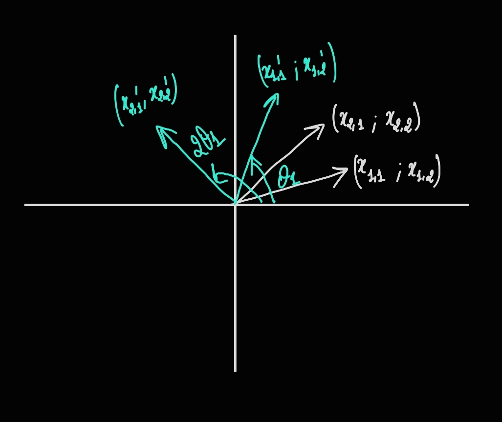
We do a similar operation as depicted in the image on all pairs of all tokens where the pairs at the same position get rotated by a multiple of the same base angle, and that multiple depends on their position in the input sequence.

This reminds of the sinusoidal position encodings where we operate on odd and even indices.

And remember, since $R_{\Theta}^{d}$ is orthogonal, it doesn’t change the norm of the vectors!

No Position Encoding (NoPE)

Paper: The Impact of Positional Encoding on Length Generalization in Transformers

The No Position Encoding’s idea is straightforward, just not using any kind of explicit position encoding method.

The NoPE paper focuses on the length generalization at downstream tasks, so they focus on the metrics of the downstream tasks instead of the language modeling perplexity.

The focus is also on decoder-only transformer models; the encoder part being equivalent to a bag of words since self-attention is invariant to permutation.

In the same idea of NoPE, the two mentioned papers Transformer Dissection: An Unified Understanding for Transformer’s Attention via the Lens of Kernel and Transformer Language Models without Positional Encodings Still Learn Positional Information show that decoder-only models perform well on in-distribution settings even without encoding positional information. So the question that is to be asked is, how well do these models generalize?

Since the goal of the paper is to evaluate the length generalization on downstream tasks, most of the experiments that were conducted were on synthetic tasks, the tasks you would typically classify as downstream tasks. They did however scale up to 1B model and train on a subset of StarCoder. Most of the PE papers conduct experiments for the length generalization on the language modeling itself so we can’t really do some kind of honest meta-analysis.

In their synthetic tasks results NoPE seems to be the better choice among the other PEs while on the language modeling task of the 1B model it seems to be bested by ALiBi. However, the performance of both methods is close in some cases of length generalization.

The reason, from what I understood, of not focusing on language modeling is that the training data for it contains a lot of short-range dependencies thanks to human cognitive constraints, so it benefits methods like ALiBi which has a bias towards recency, thus not reflecting the real length generalization capability of the model.

In the paper the authors prove two theorems, the first one is about encoding the absolute position of the tokens. The authors construct query, key, value, concatenation weight matrices of the first head of the first layer, as well as the weight matrices of the feed-forward network of the first layer, such that absolute position is computed and forwarded to the next layer. The proof does use the fact an approximation theorem so we don’t really know how wide the feed-forward network has to be. The second theorem is that there exist a parametrization of the NoPE decoder only model, or a combination of parameters if you like, such that the scaled dot-product can be written as the sum of a function of the query and key only and a function of the relative difference of the positions, that would mean that the network does encode the relative difference. That theorem does rely on the first theorem and that we can recover the absolute position encoding in the hidden state in a very specific way.

The authors also conduct some experiments where they compare the attention distributions between different heads of different networks trained with different PE encodings with the attention distributions of a NoPE network and they do find that with SGD NoPE’s attention patterns resemble the most T5’s RPE and the least APE and RoPE. You can refer to section 5.2 of the paper for the details of how they compare the attention distributions etc.

The paper also studies the influence of scratchpad, also called Chain-of-Thought on length generalization but since it’s not something that’s widely done, I will skip it.

Conclusion

ALiBi, FIRE and NoPE papers agree on the fact that RoPE isn’t great at length generalization while they also agree that T5’s RPE is a great PE (never better than their own methods though). It seems like the additive RPE methods lead to the most promising results and I’m excited to see what can be built upon FIRE. At the same time, it might be because the benchmarks are not well done. The Llama models and Mistral models all use RoPE so I’m sure it works well.

I wanted to do a meta-analysis on the results of different methods but since they train different models (scale and number of parameters) on different datasets, using different metrics (compared to RoPE or NoPE e.g.) etc. It’s hard to compare them in a fair way. The pure RPE papers might have not tuned their hyperparameters when training the models with RoPE and used the same hyperparameters that worked for their methods, which might have led to RoPE having worst results than their methods as well.

Note about the proofs in FIRE and NoPE : as it is the case for many proofs in machine learning that tie the implementation side to the theoretical side, it’s is extremely hard to confirm the theorems with experiments. For example many of the proofs in FIRE rely on the fact that we can put a upper bound on the sequence lengths (like the $L_{0}$ in the reconstruction of ALiBI with FIRE). This works as long as we can get that upper bound, which in practice we can, we don’t have infinitely large sequences, but we don’t know how much easy it is to learn such functions (not talking about the ALiBi reconstruction per se, just using it to illustrate my thoughts). Another example is how in NoPE we only have matrices of zeros and ones which are extremely hard to obtain in practice, or how the position can be recovered from $1/t$ (if $t$ is huge $1/t$ is almost $0$… needless to talk about the underflow issues etc.). This is not even mentioning how the second theorem relies on the ability to write the hidden state in a very specific way.