Transformers: Attention Is All You Need

All the code in this article can be found on ReinforcedKnowledge/deep-learning-from-scratch/transformer

Background

The Transformer comes as an answer to the sequential computation constraint that recurrent neural networks (RNNs), long short-term memory neural networks (LSTMs) and gated recurrent neural networks (GRUs) suffer form. The Transformer leverages the attention mechanism that allows to model dependencies between positions in the input and/or output sequences regardless of their distances.

Model Architecture

Attention

The description of attention by the authors of the paper is clear and concise, hence we’re citing it here:

An attention function can be described as mapping a query and a set of key-value pairs to an output, where the query, keys, values, and output are all vectors. The output is computed as a weighted sum

So we can write this as:

How do we interpret this? In the context of applying the transformer architecture to sequences of tokens, our query here is of shape (1, d), it represents something we want to know about the current element in your sequence. We want to look for this information in all the other elements of the sentence, this information is held in the $\mathbb{R}^{m\times v}$ matrix that is $V$, the values. For each element of that sentence, we have $v$ values that represent how much that element has of different “attributes”. It is important to note that this is just our interpretation and we don’t know what these “attributes” are. Why do we need the keys? Why don’t we look for the values directly? The keys are associated with other elements in the sequence as you can infer from its shape (m, d). The keys are needed since each element holds different values for the different attributes. It’s not a hard inclusion but a soft one. So we need the keys to determine how much information that other elements in the sentence will be contributing to answer the query about our initial element, they’re used to weigh the relevance of its values. That’s also why you see that the output of the attention function is a vector where each position $j$ is a weighted sum of $v_{i,j}$, we weigh the importance of the value for the attribute $j$ for different elements in the sentence with regard to our query.

Multi-Head Attention

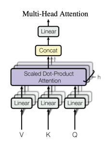
In the above figure, we suppose that we already have $Q$, $K$ and $V$. In practice, these come either from the embedded sequence or from the neural network’s previous block, so before the linear projections the queries, keys and values will be of shape (batch size, sequence length, dimension) (the dimension can be the embedding dimension or the “hidden state”, which is the output’s dimension from the feed-forward position). Let’s consider batch size = $1$, sequence length = $m$ and dimension = $d$. So at this stage we have, $Q\in\mathbb{R}^{m\times d}$, $K\in\mathbb{R}^{m\times d}$ and $V\in\mathbb{R}^{m\times d}$.

Let $h$ be the number of attention heads, we map each one of $Q,K,V$ to $h$ linear projections, we have then $h$ linear projections for $Q, K, V$, which gives us in the general case $h$ projections $P_{1}^{Q},...P_{h}^{Q}\in\mathbb{R}^{m\times q}$ for $Q$, and $P_{1}^{K},...P_{h}^{K}\in\mathbb{R}^{m\times k}$ for $K$ and $P_{1}^{V},...P_{h}^{V}\in\mathbb{R}^{m\times v}$ for $V$.
This is interesting because we can think of these dimensions $q$, $k$ and $v$ as the dimensions of space that represent the queries, the keys and values. But since we learn fixed projections, we can argue that through training these spaces will be better at targeting some kind of semantics in our sequences rather than others. When we use many heads, we have different spaces that will target different semantics.

class MultiHeadedAttention(nn.Module):
  def __init__(self, d_model=512, h=8):
    super(MultiHeadedAttention, self).__init__()
    self.d_model = d_model
    self.h = h
    self.d_k = d_model // h
    self.query_linears = nn.ModuleList([nn.Linear(d_model, self.d_k) for i in range(h)])
    self.key_linears = nn.ModuleList([nn.Linear(d_model, self.d_k) for i in range(h)])
    self.value_linears = nn.ModuleList([nn.Linear(d_model, self.d_k) for i in range(h)])
    self.projection_layer = nn.Linear(h * self.d_k, d_model)

  def forward(self, Q, K, V, mask=None):
    # First we prepare the query, key and value projections
    batch_size = Q.size(0)
    queries = torch.cat([linear(Q).view(batch_size, 1, -1, self.d_k) for linear in self.query_linears], dim=1)
    keys = torch.cat([linear(K).view(batch_size, 1, -1, self.d_k) for linear in self.key_linears], dim=1)
    values = torch.cat([linear(V).view(batch_size, 1, -1, self.d_k) for linear in self.value_linears], dim=1)

    # Now we can do the attention computation
    x = scaled_dot_product_attention(queries, keys, values, mask)

    x = x.transpose(1, 2)
    x = x.contiguous()
    x = x.view(batch_size, -1, self.h * self.d_k) # The "concat" step
    x = self.projection_layer(x)
    return x

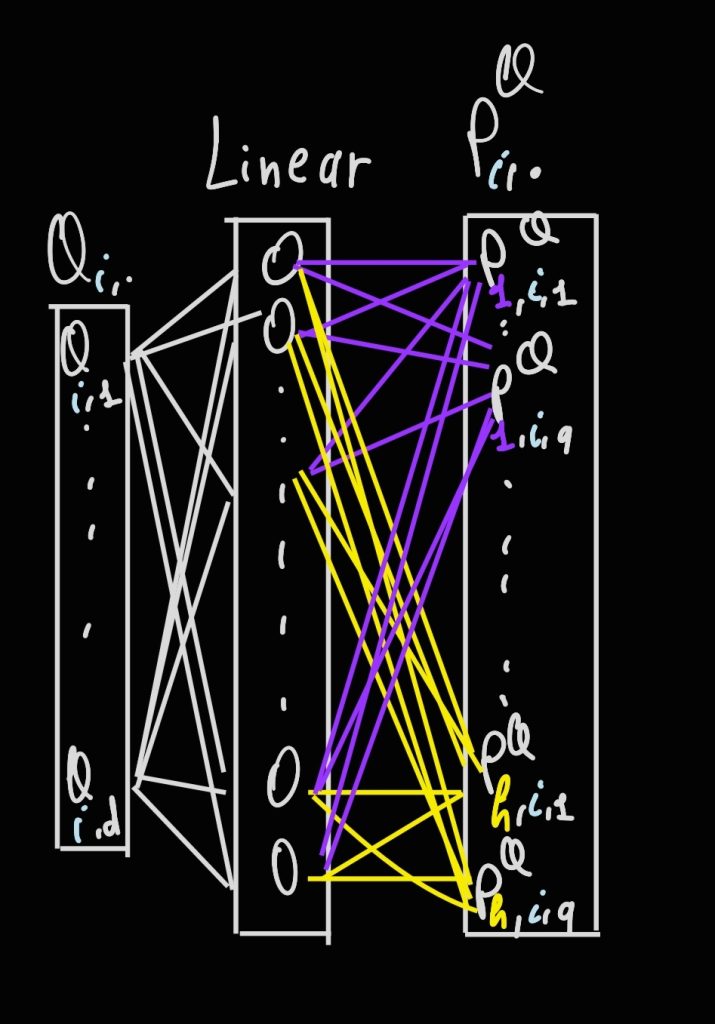
This code is is not intended to be optimal and this way of doing the Multi-Head Attention isn’t as well, but this is a faithful representation of the paper’s ideas. One easy way to improve the code and that is also used in practice is that instead of having $h$ linear layers for each of $Q$, $K$ and $V$ that produce $h$ projections for each of $Q, K, V$, we only keep $1$ linear layer for each and that will output a sort of concatenated projections. This leads to a faster computation through parallelization of the process while also reducing the memory overhead of all the projections that we were computing before. You can see with the image below that we can reshape that one big projection into $h$ smaller vectors.

So a better version of the code would be:

class MultiHeadedAttention(nn.Module):
  def __init__(self, d_model=512, h=8):
    super(MultiHeadedAttention, self).__init__()
    self.d_model = d_model
    self.h = h
    self.d_k = d_model // h

    # Using single linear layer for each query, key and value
    self.query_linear = nn.Linear(d_model, d_model)
    self.key_linear = nn.Linear(d_model, d_model)
    self.value_linear = nn.Linear(d_model, d_model)

    self.projection_layer = nn.Linear(h * self.d_k, d_model)

  def forward(self, Q, K, V, mask=None):
    batch_size = Q.size(0)

    # Apply the linear layers and split into h heads
    queries = self.query_linear(Q).view(batch_size, -1, self.h, self.d_k).transpose(1, 2)
    keys = self.key_linear(K).view(batch_size, -1, self.h, self.d_k).transpose(1, 2)
    values = self.value_linear(V).view(batch_size, -1, self.h, self.d_k).transpose(1, 2)

    # Apply scaled dot product attention
    x = scaled_dot_product_attention(queries, keys, values, mask)

    # Concatenate heads and put through final linear layer
    x = x.transpose(1, 2).contiguous().view(batch_size, -1, self.h * self.d_k)
    x = self.projection_layer(x)

    return x

The Multi-Head Attention block doesn’t end there but also contains a concat which is used to concatenate the results from each head, and a linear layer. The result of the concat will be of shape $(m, h \times v)$ and the linear layer has a weight matrix of shape $(h \times v, d)$. So after the linear layer we get back to that initial dimension $d$.

Scaled Dot-Product Attention

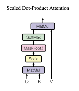
Let’s forget for the moment the scaled part of the scaled dot-product and focus on the dimensions. We have $h$ dot products, $P_{l}^{Q}(P_{l}^{K})^{T}$. We see this computation can’t work out if $q\neq k$. Let’s take $q=k=d_{k}$ now. The scaled dot-product attention is then $softmax(\frac{P_{l}^{Q}(P_{l}^{K})^{T}}{\sqrt{d_{k}}})P_{l}^{V}$.
Let’s check if this is compatible with what we’ve said before in the attention section. Inside the softmax, we have a matrix of shape (m, m). Is it the shape we’re supposed to get? Yes, because we’re relating every position in the sequence to every other position.
In order not to clutter this space, let’s check what’s happening at the $i$ th position. At the $i$ th position of the dot-product result we have the following row: $P_{l,i,.}^{Q}(P_{l,1,.}^{K})^{T}$ which is $(\sum_{j=1}^{k}P_{l,i,j}^{Q}P_{l,1,j}^{K},...,\sum_{j=1}^{k}P_{l,i,j}^{Q}P_{l,m,j}^{K})$. Is this what we’re supposed to get? Totally, inside the softmax, at row $i$, we’re supposed to have at the $j$ th position in the row a number that reflects the compatibility between the query for the position $i$ in our sequence and the key for the position $j$ in our sequence. Now, this is already compatible with the general definition of attention. I haven’t found any paper that uses this form directly to compute attention, but we’ll discuss why softmax instead of some other functions in another blog post (stay tuned 😁).

def scaled_dot_product_attention(Q, K, V, mask=None):
  scaled_dot_product = torch.matmul(Q, K.transpose(-2, -1)) / math.sqrt(K.size(-1))
  if mask is not None:
    scaled_dot_product = scaled_dot_product + mask
  attention_scores = F.softmax(scaled_dot_product, dim=-1)
  return torch.matmul(attention_scores, V)

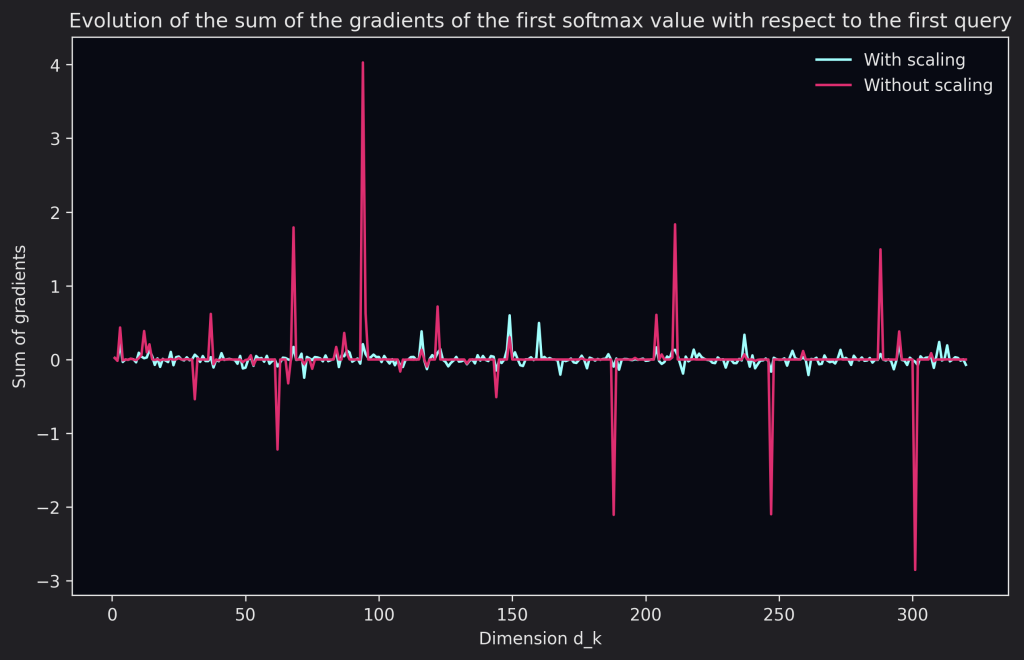
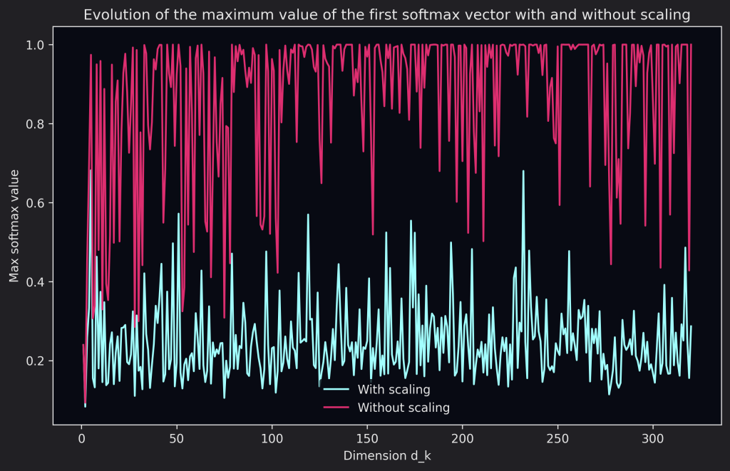
Why do we need to scale the dot-product? To rephrase what was written in the paper, large values of $d_{k}$ lead to large values in the dot-product which pushes the softmax to regions where its gradients are extremely small. The authors illustrate their claim by examining the variance of the do product between a query vector $q$ and a key vector $k$ assuming that their individual components are independent random variances with mean $0$ and variance $1$, resulting into a variance of $d_{k}$ for the dot product. It’s important to note that this issue only happens for higher values of $d_{k}$ and additive attention suffers less from this issue. We’ll talk about different attention mechanisms in another post 😁

We can visualize this behavior by randomly initializing a query and key matrices and checking the maximum value for the softmax as well as the gradients. We can see that without scaling, the gradient is almost always zero, except for the occasional peaks, while with scaling it does vary a little bit, we can also see that the softmax’ maximum value is very large and hits $1$ quite often (meaning the rest of the values are $0$) and also stays stationary around 1 quite often as well.

grads_with_scaling = []
grads_without_scaling = []
max_softmax_value_with_scaling = []
max_softmax_value_without_scaling = []
dk_values = range(1, 321)

for d_k in dk_values:
    Q = torch.randn(16, d_k, requires_grad=True)
    K = torch.randn(16, d_k, requires_grad=True)

    # Compute scaled dot product with scaling
    scaled_dot_product = torch.matmul(Q, K.T) / math.sqrt(d_k)
    softmax_value = F.softmax(scaled_dot_product, dim=-1)
    softmax_value[0, 0].backward()
    first_query_grad = Q.grad[0, :]
    grads_with_scaling.append(torch.sum(first_query_grad).item())
    max_softmax_value_with_scaling.append(torch.max(softmax_value[0, :]).item())

    Q.grad.zero_()
    K.grad.zero_()

    # Compute scaled dot product without scaling
    scaled_dot_product = torch.matmul(Q, K.T) / 1.0
    softmax_value = F.softmax(scaled_dot_product, dim=-1)
    softmax_value[0, 0].backward()
    first_query_grad = Q.grad[0, :]
    grads_without_scaling.append(torch.sum(first_query_grad).item())
    max_softmax_value_without_scaling.append(torch.max(softmax_value[0, :]).item())

    Q.grad.zero_()
    K.grad.zero_()

Masked and Causal Attention

As you may have noticed in our code for the scaled dot-product, we’re including a mask.
What is the role of a mask in the attention mechanism? Masks are used to block some positions to attend to other positions. In the transformer architecture we’re using mainly two types of masks, the causal mask; which in turn leads to the causal attention, the padding mask and the memory mask.

How does the mask work? A mask blocks certain positions by attending to others by replacing the corresponding value inside the softmax by $-\infty$. If we don’t want position $i$ to attend to position $j$ for one reason or another, we’ll just replace the dot-product inside the softmax by $-\infty$ so that its softmax value is $0$, thus it won’t contribute by its attribute value. That’s why we’re adding the mask to the dot-product, inside the softmax computation.

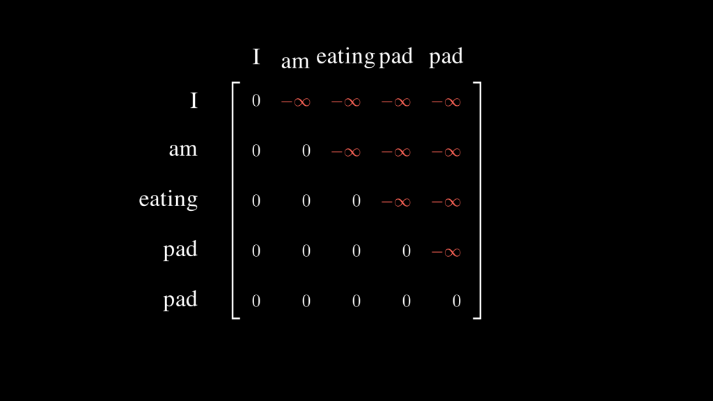
What are the causal mask and causal attention? The causal mask blocks tokens from attending to subsequent tokens, thus no token can “look ahead”. This is important in auto-regressive tasks where we predict the next token. This enables us to avoid information leakage from the future to the past where the models uses during training information that it shouldn’t have access to and won’t have access to during inference. So depending on how you set up your data, the causal mask is a triangular matrix of zeros (excluding the diagonal because an element can attend to itself) and $-\infty$.

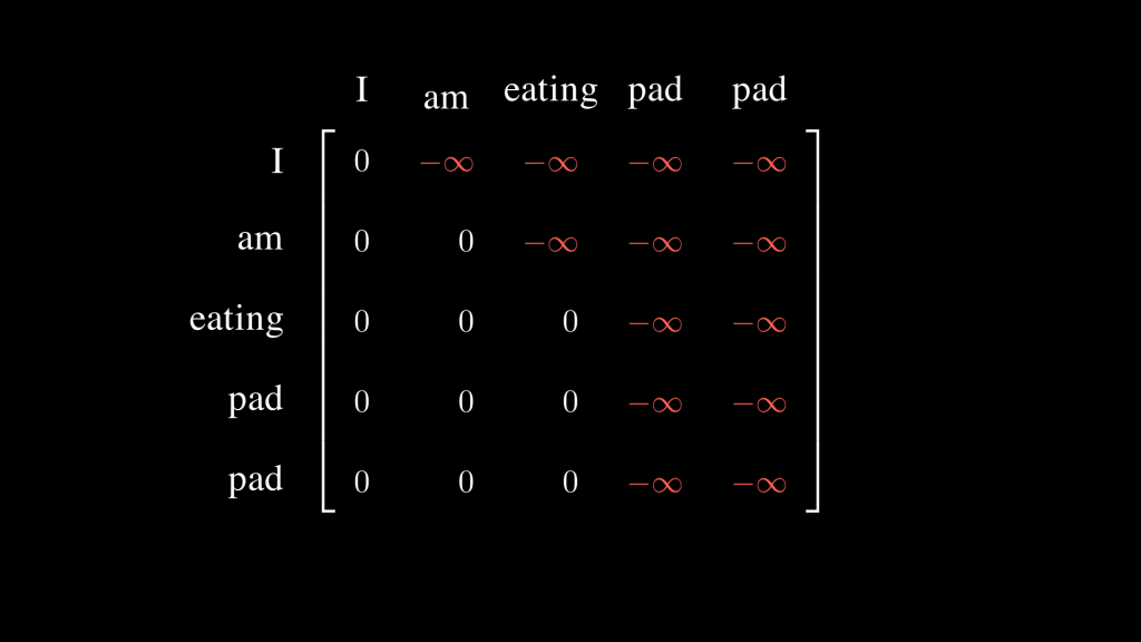
The example below shows an example of such a mask. As you can see, every token is only attending to itself and the token before it. The $-\infty$ will nullify the effect of the dot product when applying the softmax, so no token is “looking ahead”.

Note: Here I’m just showing the causal mask, but the real mask we’ll be using during training will also mask the padding tokens. We’re discussing masking the padding tokens just after this paragraph.

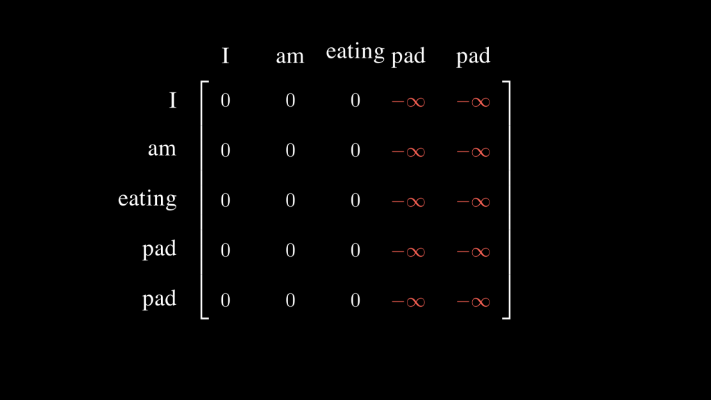
What is the padding mask? The padding mask is just a mask to block our tokens from attending to the padding tokens. Padding tokens shouldn’t be included in the attention computation since they don’t carry any information about the data and we don’t want our model to be influence by such tokens. So generally, again this will depend on your data setup, the padding masks are zeros and at there are $-\infty$ in the the last columns (which correspond to query tokens attending to the padding tokens). This way, a non padding token won’t be attending to padding tokens. We only mask the padding queries in the keys and not in the queries. Remember that queries probe the keys and the dot-product helps us determine how much each element in the sequence is relevant for other elements. So, it’s useless to compute the contribution of padding tokens with respect to non-padding tokens since padding tokens’ use isn’t to understand the tokens. But, it’s important for padding tokens to interact with other tokens, so the model knows where these padding tokens are, and that’s why we don’t mask them in the queries.

The example below shows an example of such a mask. We don’t want to change the dot product between the queries and the keys of the positions that contain useful information, which are non-padding tokens, and we want to nullify the effect the dot product between the queries and the keys associated with the padding tokens, that’s why in the mask we have $-\infty$ in the keys so when we apply the softmax these elements in the softmax result will be $0$ and won’t influence the multiplication with the values.

What is the memory mask? The memory here refers to outputs from the encoder. As we will see in the following section, the first Transformer architecture consisted of an encoder and a decoder part. The encoder encodes the input and sends it to the decoder. This output from the encoder is what we refer to as the memory. The memory mask is a mask adapted for the decoder stage that masks the padding tokens (or maybe, if the use case requires so, mask other types of tokens) in the memory. So a memory mask is just a padding mask but with a different shape, its shape is (target sequence length, input sequence length) because we don’t want our target sequence to attend to padding tokens in the source sequence.

For the sake of the example, let’s say we’re translating from English, our source language, to French, our target language. Then the shape of the memory mask, which we use at the second stage in the decoder part, is of shape (target sequence length, input sequence length) because the queries come from the decoder block and the keys come from the encoder block. We don’t want the tokens in our target language to attend to the padding tokens in our source language, so we have to mask them.

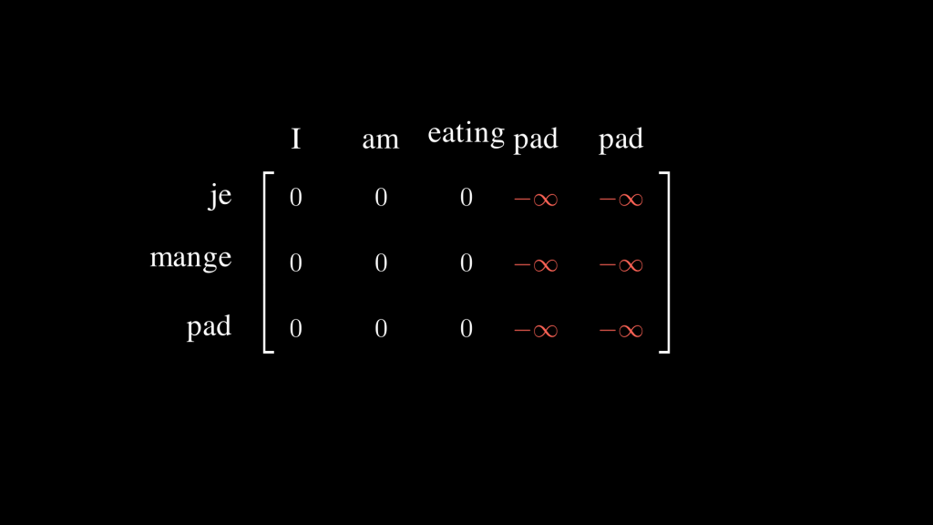
Note: The batches containing the examples from the source language and their translations to the target language don’t necessarily need to have the same maximum sequence length for the both languages, that’s why we illustrated the example that way.

Note: We can also have a combination of masks, like in the first stage of the decoder, which we will explore in the following section, we combine the padding and causal masks into one mask, that we will call the target mask. The example below illustrates this idea.

Note: This examples are for illustration purposes only, if we wanted to stay consistent then the causal masks should be in Spanish. The shapes also may or may not reflect the reality of the code since the dot-product also contains the batch size and number of heads dimensions, so whether we’re using broadcasting or not the shapes may vary, but the essence of the masks are what the examples illustrate.

For a better understanding of masks, let’s write code for our own masks. Since the masks are added to the dot-product, we want them to have the same shapes, and since we’re doing a dot-product between two matrices of shape (seq length, $d_k$) then the dot-product’s shape is (seq length, seq length), but we’re also doing that for each head in parallel so the shape is ($h$, seq length, seq length) and we’re doing that for each example so the final shape of the dot-product is (batch size, $h$, seq length, seq length). Our masks must have the same shapes. At the second stage of the decoder part of the transformer, we’re doing a dot-product between queries coming from the decoder, so a shape (target sequence length, $d_k$) and keys coming from the encoder, so a shape (input sequence length, $d_k$), that’s why at this stage the mask will have a shape of (batch size, $h$, target seq length, source seq length). We mean by source and target here the source language, the inputs to the encoder part of the transformer, and the target language which are the inputs to the decoder part of the transformer.
Now, the masks only depend on the tokens in the sequence, so we can create, for each sequence in the batch, the masks for the shape $(seq\ length, seq\ length)$, or $(target\ seq\ length, source\ seq\ length)$, and then repeat that across the heads.

Let’s say we’re translating from English to French and that our batch consists of the two following examples and tokens:

src_sentences = torch.tensor([
  [1, 2, 3, 0, 0],  # I am eating pad pad
  [4, 5, 6, 0, 0]   # I like blogging pad pad
])

tgt_sentences = torch.tensor([
  [1, 2, 3, 4, 5, 6, 0, 0, 0], # Je suis en train de manger pad pad pad
  [1, 7, 9, 0, 0, 0, 0, 0, 0]  # Je aime blogger pad pad pad pad pad pad
])

Let’s create a function that returns the padding mask and let’s try it on our source sentences. So, for the padding mask we can take the batch consisting of tokens, and wherever there are padding tokens we’ll fill in with $-\infty$. Doing that, we just need to expand that to the correct shape that’s used by the model in its multi-head attention block. Since we’re able to do that, we can do it for both the source batch and the target batch and combine both masks which will help us mask padding tokens coming from both batches in the second stage of the decoder part of the model.

def create_padding_mask(src_sentences, tgt_sentences, pad=0, Nheads=8):
    _, src_seq_length = src_sentences.shape
    tgt_batch_size, tgt_seq_length = tgt_sentences.shape

    memory_mask = torch.zeros(tgt_batch_size, Nheads, tgt_seq_length, src_seq_length)

    # Create masks for positions where src_sentences and tgt_sentences are equal to pad
    src_pad_mask = src_sentences == pad

    # Expand the src_pad_mask to match the size (batch_size, 1, 1, src_seq_length)
    src_pad_mask_expanded = src_pad_mask.unsqueeze(1).unsqueeze(2)
    src_pad_mask_expanded = src_pad_mask_expanded.expand(tgt_batch_size, Nheads, tgt_seq_length, src_seq_length)

    # Apply the mask to the memory mask
    memory_mask.masked_fill_(src_pad_mask_expanded, -float('inf'))

    return memory_mask

def create_src_masks(src_sentences, pad, Nheads=8):
  return create_padding_mask(src_sentences, src_sentences, pad, Nheads)

create_src_masks(src_sentences, 0).size()
# torch.Size([2, 8, 5, 5])

create_src_masks(src_sentences, 0)[0, 0, :, :]
# tensor([[0., 0., 0., -inf, -inf],
#         [0., 0., 0., -inf, -inf],
#         [0., 0., 0., -inf, -inf],
#         [0., 0., 0., -inf, -inf],
#         [0., 0., 0., -inf, -inf]])

We can create the same padding mask but for the target sentences:

create_padding_mask(tgt_sentences, tgt_sentences, pad=0).size()
# torch.Size([2, 8, 9, 9])

create_padding_mask(tgt_sentences, tgt_sentences, pad=0)[0, 0, :, :]
# tensor([[0., 0., 0., 0., 0., 0., -inf, -inf, -inf],
#         [0., 0., 0., 0., 0., 0., -inf, -inf, -inf],
#         [0., 0., 0., 0., 0., 0., -inf, -inf, -inf],
#         [0., 0., 0., 0., 0., 0., -inf, -inf, -inf],
#         [0., 0., 0., 0., 0., 0., -inf, -inf, -inf],
#         [0., 0., 0., 0., 0., 0., -inf, -inf, -inf],
#         [0., 0., 0., 0., 0., 0., -inf, -inf, -inf],
#         [0., 0., 0., 0., 0., 0., -inf, -inf, -inf],
#         [0., 0., 0., 0., 0., 0., -inf, -inf, -inf]])

But to complete the mask for the decoder part we also need a causal mask

def create_lookahead_mask(sentences, Nheads=8):
  batch_size, sequence_length = sentences.shape
  mask = torch.ones(sequence_length, sequence_length).triu(diagonal=1)
  mask = mask.masked_fill(mask == 1, -float('inf'))
  mask = mask.unsqueeze(0).unsqueeze(0).expand(batch_size, Nheads, -1, -1)
  return mask

create_lookahead_mask(tgt_sentences).size()
# torch.Size([2, 8, 9, 9])

create_lookahead_mask(tgt_sentences)[0, 0, :, :]
# tensor([[0., -inf, -inf, -inf, -inf, -inf, -inf, -inf, -inf], Je -> Je
#         [0., 0., -inf, -inf, -inf, -inf, -inf, -inf, -inf], suis -> Je suis
#         [0., 0., 0., -inf, -inf, -inf, -inf, -inf, -inf], en -> Je suis en
#         [0., 0., 0., 0., -inf, -inf, -inf, -inf, -inf], train -> Je suis en train
#         [0., 0., 0., 0., 0., -inf, -inf, -inf, -inf], de -> Je suis en train de 
#         [0., 0., 0., 0., 0., 0., -inf, -inf, -inf], manger -> Je suis en train de manger
#         [0., 0., 0., 0., 0., 0., 0., -inf, -inf],
#         [0., 0., 0., 0., 0., 0., 0., 0., -inf],
#         [0., 0., 0., 0., 0., 0., 0., 0., 0.]])

As you can see, with the causal mask non-padding tokens will automatically not attend to padding tokens, but we still need to mask the padding tokens so that the other padding tokens don’t attend to them. You can see how each token is attending only to the tokens up to its position.

def create_tgt_masks(tgt_sentences, pad, Nheads=8):
  lookahead_mask = create_lookahead_mask(tgt_sentences, Nheads)
  padding_mask = create_padding_mask(tgt_sentences, tgt_sentences, pad, Nheads)
  return lookahead_mask + padding_mask

create_tgt_masks(tgt_sentences, pad=0).size()
# torch.Size([2, 8, 9, 9])

create_tgt_masks(tgt_sentences, pad=0)[0, 0, :, :]
# tensor([[0., -inf, -inf, -inf, -inf, -inf, -inf, -inf, -inf],
#         [0., 0., -inf, -inf, -inf, -inf, -inf, -inf, -inf],
#         [0., 0., 0., -inf, -inf, -inf, -inf, -inf, -inf],
#         [0., 0., 0., 0., -inf, -inf, -inf, -inf, -inf],
#         [0., 0., 0., 0., 0., -inf, -inf, -inf, -inf],
#         [0., 0., 0., 0., 0., 0., -inf, -inf, -inf],
#         [0., 0., 0., 0., 0., 0., -inf, -inf, -inf],
#         [0., 0., 0., 0., 0., 0., -inf, -inf, -inf],
#         [0., 0., 0., 0., 0., 0., -inf, -inf, -inf]])

Below is the code for creating a memory mask, you can also see how the mask will only consider the dot-product between the queries coming from the decoder and the non-padding tokens’ keys coming from the encoder part

def create_memory_masks(src_sentences, tgt_sentences, pad, Nheads=8):
  return create_padding_mask(src_sentences, tgt_sentences, pad, Nheads)

create_memory_masks(src_sentences, tgt_sentences, pad=0).size()
# torch.Size([2, 8, 9, 5])

create_memory_masks(src_sentences, tgt_sentences, pad=0)[0, 0, :, :]
# tensor([[0., 0., 0., -inf, -inf],
#         [0., 0., 0., -inf, -inf],
#         [0., 0., 0., -inf, -inf],
#         [0., 0., 0., -inf, -inf],
#         [0., 0., 0., -inf, -inf],
#         [0., 0., 0., -inf, -inf],
#         [0., 0., 0., -inf, -inf],
#         [0., 0., 0., -inf, -inf],
#         [0., 0., 0., -inf, -inf]])

We can check if the masks work when we apply softmax.

Nheads = 8
d_model = 512

batch_size, src_seq_length = src_sentences.shape
_, tgt_seq_length = tgt_sentences.shape

queries = torch.randn(batch_size, Nheads, tgt_seq_length, d_model)
keys = torch.randn(batch_size, Nheads, src_seq_length, d_model)

def softmax_scaled_dot_product(Q, K, mask=None):
  scaled_dot_product = torch.matmul(Q, K.transpose(-2, -1)) / math.sqrt(K.size(-1))
  if mask is not None:
    scaled_dot_product = scaled_dot_product + mask
  return F.softmax(scaled_dot_product, dim=-1)

softmax_scaled_dot_product(queries, keys, create_memory_masks(src_sentences, tgt_sentences, pad=0))[0, 0, :, :]
# tensor([[0.1468, 0.3032, 0.5501, 0.0000, 0.0000],
#         [0.1019, 0.5245, 0.3736, 0.0000, 0.0000],
#         [0.4444, 0.4587, 0.0969, 0.0000, 0.0000],
#         [0.0977, 0.8538, 0.0485, 0.0000, 0.0000],
#         [0.3260, 0.4940, 0.1800, 0.0000, 0.0000],
#         [0.6682, 0.0374, 0.2944, 0.0000, 0.0000],
#         [0.2788, 0.1720, 0.5492, 0.0000, 0.0000],
#         [0.3008, 0.2414, 0.4578, 0.0000, 0.0000],
#         [0.3741, 0.5486, 0.0773, 0.0000, 0.0000]])

As we can see, after applying the mask, the softmax value for the masked positions is $0$.

Note: It is important to keep in mind that the mask is the same across the heads for the same batch element.

Encoder and Decoder Stacks

The original transformer architecture is composed of an encoder part and a decoder part. This architecture design is similar to what was used before for neural machine translation and many other sequence to sequence use cases. As the name suggests, the encoder part is responsible to encode, creating a meaningful representation of the input sequences, and the decoder is responsible to decode that representation and generate the output.

The original transformer architecture is:

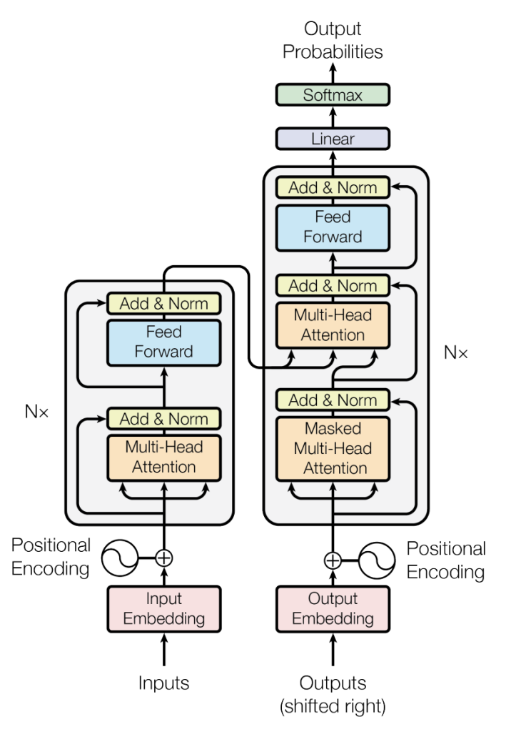
The encoder and decoder are respectively the left and right parts of that architecture:

Note: All layers and sub-layers produce outputs of the same dimension $d_{model}=512$.

About the Encoder:

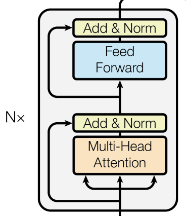
It is composed of $N = 6$ identical stacks. Each stack is composed of 2 sub-layers. The first sub-layer is the multi-head attention and the second sub-layer is a feed-forward network composed of two layers which the authors call Position-wise Feed-Forward Networks, probably because they’re applied to each position of the sequence. (Remember, the inputs of the transformer architecture are of shape $(batch\ size, source\ sequence\ length, d_{model})$ and this shape is propagated through the network, so when this shape is the input of the feed-foward network, its layers are applied along the last dimension only so we’re really using the feed-forward on each position). Both sub-layers have around them residual connections that connect to an “Add & Norml” layer where we add the output of the sub-layer to its input due to the residual connection, then we use layer norm.

The outputs of the encoder are used in the decoder.

About the Decoder:

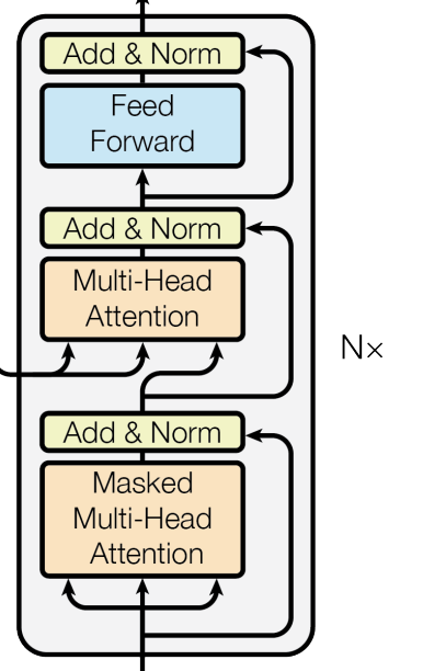
The decoder’s architecture is somewhat similar to the encoder. It is also composed of $N = 6$ identical stacks. Each stack is composed of 3 sub-layers. The first sub-layer is the masked multi-head attention, as we discussed earlier we’re using here a causal mask to block positions from looking ahead. The second layer is a multi-head attention but now we’re using the output from the encoder as keys and values, where the outputs from the masked multi-head attention are used as queries. The third sub-layer is a position-wise feed-forward network. Again, all sub-layers have around them residual connections that connect to an “Add & Norml” layer.

About the inputs of the transformer architecture:

It’s important to remember that since the original transformer architecture was used in a supervised learning fashion, so it has inputs $X$ and outputs $Y$. The use case of the paper was neural machine translation, so the inputs are sequences from a source language and the outputs are their translations, so sequences from a target language. Through there are only one set of inputsto the whole model. Throughout the article I have used the word “input” when talking about what enters a decoder, but one should keep in mind that what enters the decoder are the outputs of the transformer. We’ll talk later on about training and inference, but you may have noticed from the transformer architecture screenshot, the authors have used Outputs (shifted right) to describe what enters the decoder. It’s because when just starting the translation, the decoder should not rely on the first word in the translation to produce some output, so we shift the output to the right and give the decoder what we call a beginning-of-sentence (BOS) token indicating that we’re at the beginning of the sentence. When the decoder takes that information, along the outputs from the encoder, and gives us something in return (its output), then we can feed it a combination of both the BOS token and its output. For example, when translating the french “I eat”, at step $0$, the decoder will take the BOS token along the output of the encoder and generate something, hopefully “Je”. Then at step $1$, the decoder will take both the BOS token and the token associated with “Je”, and again the output of the encoder, to generate a second word, hopefully $mange$. At the next step, the decoder will take both the BOS token, the token associated with “Je”, the token associated with “mange”, and the output of the encoder and should generate what we call an end-of-sentence (EOS) token, indicating that we have finished.
In general, especially in the first stages of training, the decoder won’t generate the correct words so we apply a strategy called teacher forcing where instead of feeding it the result of its output, we feed it the correct translation. That way the model will struggle because it won’t propagate as much errors as in the other case.
So that’s why the authors are using the term “outputs (shifted right)” when talking about what enters the decoder, because we’re taking those entries from the outputs, and they’re shifted to the right because of the nature of the problem and training.

Note: Don’t confuse teacher forcing with the causal mask. The causal mask is a way to make tokens attend only to positions up to theirs while teacher forcing just means instead of using the outputs from the model we’re going to use the tokens in the $y$ sentence.

Before coding the Encoder and Decoder parts of the Transformer, let’s delve into the Position-wise Feed Forward Networks because they’re used as sub-layers.

Position-wise Feed-Forward Networks

The position-wise feed-forward network (refer to this, for an explanation of the name) is a fully-connected neural network composed of two linear layers where the first has dimensionality $d_{ff} = 2048$ (in general this dimension is equal to $4 \times d_{model}$) and with a ReLU activation function while the second layer is a linear layer with dimensionality $d_{model}$ (as we said before, all sub-layers’ outputs have this dimension), so it doesn’t have an activation function.

Now we can code both the encoder and the decoder, we’ll be using the MultiHeadAttention class defined earlier

class PositionWiseFeedForward(nn.Module):
  def __init__(self, d_model=512, d_ff=2048):
    super(PositionWiseFeedForward, self).__init__()
    self.linear1 = nn.Linear(d_model, d_ff)
    self.linear2 = nn.Linear(d_ff, d_model)

  def forward(self, x):
    x = self.linear1(x)
    x = F.relu(x)
    return self.linear2(x)
  
class Encoder(nn.Module):
  def __init__(self, d_model=512, h=8, d_ff=2048, dropout=0.1):
    super(Encoder, self).__init__()
    self.multi_headed_attention = MultiHeadedAttention(d_model, h)
    self.position_wise_feed_forward = PositionWiseFeedForward(d_model, d_ff)
    self.layernorm1 = nn.LayerNorm(d_model)
    self.layernorm2 = nn.LayerNorm(d_model)
    self.dropout = nn.Dropout(p=dropout)

  def forward(self, x, mask=None):
    # MHA
    mha_output = self.dropout(self.multi_headed_attention(x, x, x, mask))
    # Add + Norm
    x = self.layernorm1(x + mha_output)
    # FF
    ff_output = self.dropout(self.position_wise_feed_forward(x))
    # Add + Norm
    x = self.layernorm2(x + ff_output)
    return x
  
class Decoder(nn.Module):
  def __init__(self, d_model=512, h=8, d_ff=2048, dropout=0.1):
    super(Decoder, self).__init__()
    self.masked_multi_headed_attention = MultiHeadedAttention(d_model, h)
    self.multi_headed_attention = MultiHeadedAttention(d_model, h)
    self.position_wise_feed_forward = PositionWiseFeedForward(d_model, d_ff)
    self.layernorm1 = nn.LayerNorm(d_model)
    self.layernorm2 = nn.LayerNorm(d_model)
    self.layernorm3 = nn.LayerNorm(d_model)
    self.dropout = nn.Dropout(p=dropout)

  def forward(self, x, decoder_mask, encoder_stack_output, memory_mask):
    # MMHA
    mmha_output = self.dropout(self.masked_multi_headed_attention(x, x, x, decoder_mask))
    # Add + Norm
    x = self.layernorm1(x + mmha_output)
    # MHA
    mha_output = self.dropout(self.multi_headed_attention(x, encoder_stack_output, encoder_stack_output, memory_mask))
    # Add + Norm
    x = self.layernorm1(x + mha_output)
    # FF
    ff_output = self.dropout(self.position_wise_feed_forward(x))
    # Add + Norm
    x = self.layernorm2(x + ff_output)
    return x

How Attention is Used in the Transformer

We talked about how attention is used in different parts of the transformer, so this part will be a summary of that, and also I was trying to respect the layout of the paper…

So attention is used in three different ways across the architecture:

Self-attention in the encoder part of the model where each position of an input sequence attends to all different positions of the same sequence. The queries, keys and values all come from the same place here as stated in the paper, which just means either from the embedding layer or from the previous layer of the encoder (the result of the add-norm layer on the position-wise feed-foward of the previous layer). Self-attention this way helps understand the structure of the input sequences.

Causal self-attention in the first masked multi-head attention of the decoder. This is applied on the outputs shifted to the right; the entries of the decoder. We call it self-attention because the queries, keys and values come from the outputs themselves, and we call it causal because we’re using a causal mask that allows a position to attend to positions only up to itself. This helps the decoder understand what it has generated (or if you prefer, translated).

“Cross” attention in the second multi-head attention of the decoder. I’m not sure the “cross” name is used for this, but in many multi-modal models where attention is applied on both modalities the world “cross” is used to indicate that we’re applying attention on two different modalities. I’m using the word “cross” here just to indicate that the queries, keys and values don’t come from the same place. The queries come from the previous sub-layer of the decoder, which is the causal self-attention, but the keys and values come from the encoder. Here every token in the output (shifted to the right) attends to every token in the input, this helps take into account the input, as well what has been generated, to continue generating relevant outputs.

Embeddings and Softmax

As you can see in the Transformer architecture, we have two embedding layers, one for the inputs (the source sentences) and one for the outputs (the target sentences). There’s also a linear layer after the decoder part and then a softmax is applied.

In a general setting, the input embedding layer converts a batch of inputs of shape $(n, m_{in})$ where $n$ is the batch size and $m_{in}$ is the max sequence length in that batch to a batch of shape $(n, m_{in}, d_{model})$. The input sequences are sequences of integers (tokens) and each token is associated to an embedding vector. So the weight matrix of that input embedding layer should be of size $(input\ vocab\ size, d_{model})$.

The output embedding layer functions similarly but its weight matrix is of size $(output\ vocab\ size, d_{model})$.

The linear pre-softmax layer transforms the output of the decoder from a shape $(n, m_{out}, d_{model})$ to $(n, output\ vocab\ size)$ so that when applying the softmax we get the probability of each output token.

In a general setting, there’s no rule to share the weights between these three layers. But in the original transformer architecture these layers were shared, which means that we’re using the same weights for all three layers and updating one set of weights. So we must have $input\ vocab\ size\ = target\ vocab\ size$. Beyond reducing the size of the model by now having one set of weights instead of three and the potential regularization effect that weight sharing has by learning a robust representation since the weights are used at different stages of the model, the reason put forward by the authors is the result from the paper Using the Output Embedding to Improve Language Models by Ofir Press and Lior Wolf where they find that tying the output embedding matrix in neural network language models to the input embedding matrix does improve performance.

I think this technique makes sense when using languages that share some kind of similarities. In the original transformer the use cases were translations between English and German, and English and French and these languages share a lot of similarities beyond the common latin alphabet (especially English and German). Since sharing the same weights makes all the embeddings live in the same space, I think in this case the semantics learned by the embeddings are improved.

The tokenizer used is byte-pair encoding that has a shared vocabulary between the source and target languages.
A tokenizer is a function that transforms characters, words, sentences etc. to tokens. We’ll delve into the functioning of tokenizers and the different algorithms in an upcoming post.

The authors also scale the embedding vectors by $\sqrt{d_{model}}$. The wording used is “In the embedding layers, we multiply those weights by $\sqrt{d_{model}}$” but it’s not really those shared weights of the embedding layers that are scaled.

As to why this is done, there’s no clear answer and/or proof or experiment. People hypothesized many reasons as one can find in the links referenced in this and this links. The hypotheses are:

• Not needed.
• Rescaling to accommodate the positional embeddings that we will discuss in the next section. Many say that the goal is to make the embeddings initially bigger than the positional encoding.
• To accommodate the sharing of the weights between the two embedding layers and the pre-softmax activation layer.

Positional Encoding

By design the Transformer architecture doesn’t make any assumption on the position of the tokens in, sequence it’s processing. As you can see in the attention mechanism, all tokens are processed in parallel. Whether the input is “That guy ate a pizza” or “A pizza ate that guy”, in the attention mechanism it’s all the same.

This reminds of the paper Convolutional Neural Networks on Randomized Data where they find that whether you train an MLP for classification on an image dataset (MNIST etc.), or a pixel-wise permutation of that set, the performance is going to be the same. But it’s not the case for CNNs where the performance degrades when you train them on the permuted set. This is because CNNs by design capture spatial hierarchies and local patterns in images, such as edges and textures, which are disrupted in pixel-wise permuted images but it’s not what the MLP does.

RNNs also maintain information about the order in the sequence they process since by design they process the sequence in a sequential manner, one token at a time. They also maintain a memory of the past which gives them a sense of order.

So going back to our example, for an RNN it’s different if in the past there were the words “That guy” before the word “ate” than if the words were “A pizza”. The same for a CNN it’s different if around the word “ate” there are the words “guy” and “a”, than if there are “pizza” and “that”. But in the eyes of a Transformer, it’s all the same, because it relies only on feed-forward networks and the attention mechanism.

As the authors state there are many ways to encode the position, since we’re discussing the original paper we’re going to explain what their choice was:

So what this means, is that for each position $pos$ in a given sentence, the value for each pair position in its positional encoding vector, which is of same size as the embedding vector $d_{model}$, is computed using formula $(1)$ and the value for each impair position is computed using formula $(2)$.

If we consider the 6 first dimensions (starting from $0$) of the example “I am eating a pizza” we get:

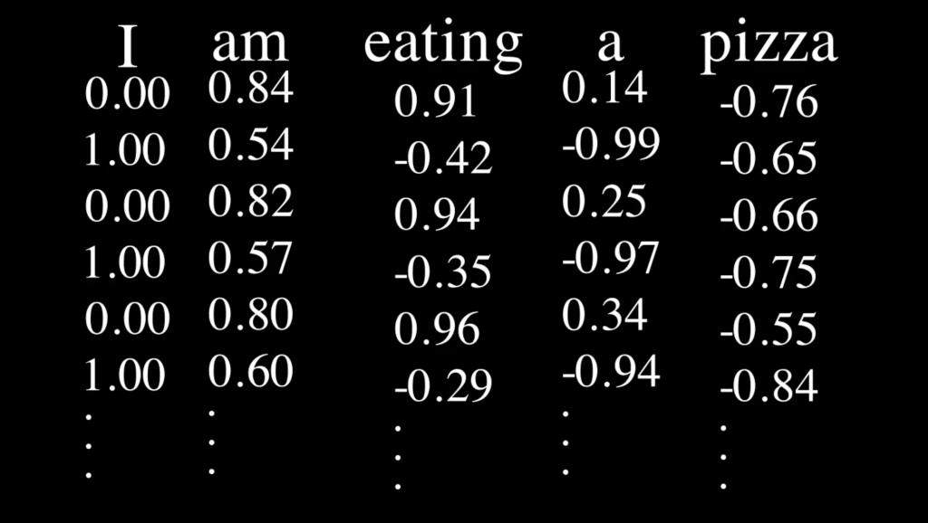
This is how the values for each of the $6$ first dimensions change across the positions in a sequence. We also show the values of the first 5 positions which are the values are the top of the red dotted lines. The plots are for $d_{model}=512$.

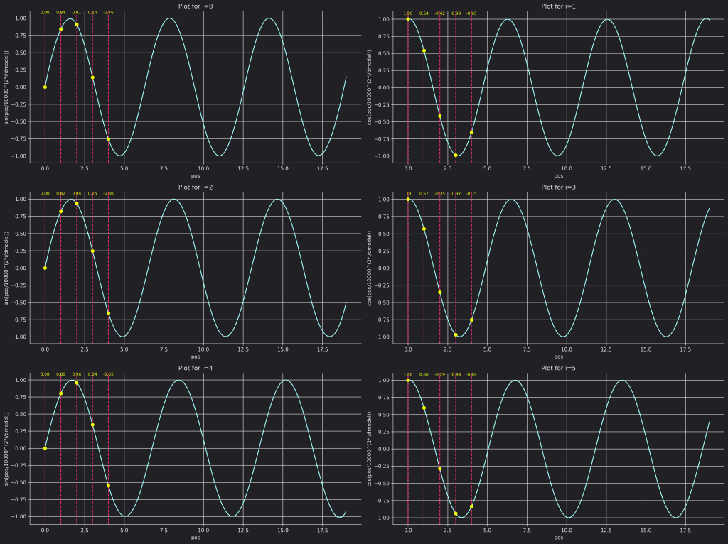
As you can notice from the formula, each dimension is a periodic function with its own frequency. Theoretically, you can’t have the same positional encoding vector for two different positions but one can notice that if $pos >> 1000^{\frac{2i}{d_{model}}}$ then the values will be the same. For extremely long sequences this type of encoding doesn’t help, but it’s hard to reach those types of lengths in practical applications.

We’ll see in an upcoming post though that this way of encoding positions doesn’t help the model generalize well beyond the maximum sequence length (context) it has seen in its training.

Let’s code both the Embedding component of our transformer architecture as well as the positional encodings

def compute_positional_encoding(max_input_tokens, d_model):
  positional_encoding = torch.zeros((max_input_tokens, d_model))
  positions = torch.arange(max_input_tokens)
  indices = torch.arange(d_model // 2)
  
  positional_encoding[:, ::2] = torch.sin(positions[:, None] / (10000 ** (2 * indices / d_model)))
  positional_encoding[:, 1::2] = torch.cos(positions[:, None] / (10000 ** (2 * indices / d_model)))
  return positional_encoding

class EmbeddingsComponent(nn.Module):
  def __init__(self, d_model, vocab, pe, dropout=0.1):
    super(EmbeddingsComponent, self).__init__()
    self.d_model = d_model
    self.positional_encoding = pe
    self.embed_layer = nn.Embedding(vocab, d_model)
    self.dropout = nn.Dropout(dropout)

  @property
  def embeddings_matrix(self):
    return self.embed_layer.weight

  def forward(self, x):
    x = self.embed_layer(x) * math.sqrt(self.d_model)
    x += self.positional_encoding[:x.size(1), :]
    return self.dropout(x)

Shapes and operations flow

I tried to synthesize in some kind of “flow” the operations and shapes at different stages of the transformer. In the following, we’ll use $i$ to denote the number of the stack of the encoder or the decoder.

We start by the encoder:

1. $X_{source}$: Source batch of shape $(n, m)$ where $n$ is the batch size and $m$ is the maximum sequence length in the batch
2. Embedding layer $X_{source}:(n, m)) \mapsto X_{emb}: (n, m, d_{model})$ create embedding vectors for the tokens in the sequence
3. Positional encoding $X_{emb}: (n, m, d_{model}) \mapsto X_{0} := X_{emb} + PE : (n, m, d_{model})$: sum the embedding vectors with the positional encodings
4. Repeat $N=6$ $X_{i} : (n, m, d_{model}) \mapsto X_{i+1} = Encoder(X_{i}) : (n, m, d_{model})$
   1. Multi-Head Attention
      • Linear $X_{i} : (n, m, d_{model}) \mapsto Q_{i} = reshaped\_(X_{i}W_{i}^{Q}) : (n, h, m, d_{k})$ we multiply the input to the first sub-layer of the Encoder by $W_{i}^{Q}$ of shape $(d_{model}, h\times d_{k})$ then we reshape to $(n, h, m, d_{k})$ so that the attention is computed on the positions
      • Linear $X_{i} : (n, m, d_{model}) \mapsto K_{i} = reshaped\_(X_{i}W_{i}^{K}) : (n, h, m, d_{k})$ we multiply the input to the first sub-layer of the Encoder by $W_{i}^{K}$ of shape $(d_{model}, h\times d_{k})$ then we reshape to $(n, h, m, d_{k})$
      • Linear $X_{i} : (n, m, d_{model}) \mapsto V_{i} = reshaped\_(X_{i}W_{i}^{V}) : (n, h, m, d_{v})$ we multiply the input to the first sub-layer of the Encoder by $W_{i}^{V}$ of shape $(d_{model}, h\times d_{v})$ then we reshape to $(n, h, m, d_{v})$
      • (Masked) Scaled-dot product $(Q_{i}, K_{i}, M) : ((n, h, m, d_{k}), ., .) \mapsto S_{i} = \frac{Q.K^{T} + M}{\sqrt{d_{k}}} : (n, h, m, m)$
      • Attention $S_{i} : (n, h, m, m) \mapsto A_{i} = softmax(S_{i}).V_{i} : (n, h, m, d_{v})$
      • Concat $A_{i} : (n, h, m, d_{v}) \mapsto Concat_{i} : (n, m, h\times d_{v})$
      • Linear $Concat_{i} : (n, m, h\times d_{v}) \mapsto MHA_{i} = Concat_{i} W_{i}^{O} : (n, m, d_{model})$ here we project the concatenated outputs from the attention heads using a multiplication by a matrix of shape $(h\times d_{v}, d_{model})$
   2. Add & Norm $(X_{i}, MHA_{i}) : ((n, m, d_{model}), .) \mapsto add\_norm\_mha_{i} = LayerNorm(X_{i} + MHA_{i}) : (n, m, d_{model})$ here we’re using the input to the encoder through a skip connection to add it to the output of the multi-head attention and apply layer norm.
   3. Point-wise feed forward $add\_norm\_mha_{i} : (n, m, d_{model}) \mapsto FF_{i} = max(0, add\_norm\_mha_{i}W_{i}^{FF, 1} + b_{i}^{FF, 1})W_{i}^{FF, 2} + b_{i}^{FF, 2} : (n, m, d_{model})$ this is a feed-forward network with two hidden layers, the first one has weights and biases $W_{i}^{FF, 1}, b_{i}^{FF, 1}$ of shape $(d_{model}, d_{ff})$ and $(1, d_{ff})$ respectively, and it uses ReLU as an activation function. While the second layer has weights and biases $W_{i}^{FF, 2}, b_{i}^{FF, 2}$ of shape $(d_{ff}, d_{model})$ and $(1, d_{model})$ and doesn’t use an activation function
   4. Add & Norm $(add\_norm\_mha_{i}, FF_{i}) : ((n, m, d_{model}), .) \mapsto X_{i+1} = LayerNorm(add\_norm\_mha_{i}, FF_{i}) : (n, m, d_{model})$

At this stage we keep in memory the outputs from the encoder $E_{5} : (n, m_{s}, d_{model})$, we use $m_{s}$ to indicate the maximum sequence length in the source batch, because it might be different in the target batch.

1. $Y_{target}$: target batch of shape $(n, m)$ where $n$ is the batch size and $m$ is the maximum sequence length in the batch
2. Embedding layer $Y_{target}:(n, m)) \mapsto Y_{emb}: (n, m, d_{model})$ create embedding vectors for the tokens in the sequence
3. Positional encoding $Y_{emb}: (n, m, d_{model}) \mapsto Y_{0} := Y_{emb} + PE : (n, m, d_{model})$: sum the embedding vectors with the positional encodings
4. Repeat $N=6$ $Y_{i} : (n, m, d_{model}) \mapsto Y_{i+1} = Decoder(Y_{i}, E_{5}) : (n, m, d_{model})$ the decoder also takes in its inputs the output from the encoder
   1. Masked Multi-Head Attention
      • Linear $Y_{i} : (n, m, d_{model}) \mapsto Q_{i} = reshaped\_(Y_{i}W_{i}^{Q}) : (n, h, m, d_{k})$ we multiply the input to the first sub-layer of the Decoder by $W_{i}^{Q}$ of shape $(d_{model}, h\times d_{k})$ then we reshape to $(n, h, m, d_{k})$ so that the attention is computed on the positions
      • Linear $Y_{i} : (n, m, d_{model}) \mapsto K_{i} = reshaped\_(Y_{i}W_{i}^{K}) : (n, h, m, d_{k})$ we multiply the input to the first sub-layer of the Decoder by $W_{i}^{K}$ of shape $(d_{model}, h\times d_{k})$ then we reshape to $(n, h, m, d_{k})$
      • Linear $Y_{i} : (n, m, d_{model}) \mapsto V_{i} = reshaped\_(Y_{i}W_{i}^{V}) : (n, h, m, d_{v})$ we multiply the input to the first sub-layer of the Decoder by $W_{i}^{V}$ of shape $(d_{model}, h\times d_{v})$ then we reshape to $(n, h, m, d_{v})$
      • Masked Scaled-dot product $(Q_{i}, K_{i}, M) : ((n, h, m, d_{k}), ., .) \mapsto S_{i} = \frac{Q.K^{T} + M}{\sqrt{d_{k}}} : (n, h, m, m)$ here we’re using the lookahead mask that we’ve talked about earlier
      • Attention $S_{i} : (n, h, m, m) \mapsto A_{i} = softmax(S_{i}).V_{i} : (n, h, m, d_{v})$
      • Concat $A_{i} : (n, h, m, d_{v}) \mapsto Concat_{i} : (n, m, h\times d_{v})$
      • Linear $Concat_{i} : (n, m, h\times d_{v}) \mapsto MHA_{i} = Concat_{i} W_{i}^{O} : (n, m, d_{model})$ here we project the concatenated outputs from the attention heads using a multiplication by a matrix of shape $(h\times d_{v}, d_{model})$
   2. Add & Norm $(Y_{i}, MHA_{i}) : ((n, m, d_{model}), .) \mapsto add\_norm\_mha_{i} = LayerNorm(Y_{i} + MHA_{i}) : (n, m, d_{model})$
   3. Masked Multi-Head Attention
      • Linear $add\_norm\_mha_{i} : (n, m, d_{model}) \mapsto cross\_Q_{i} = reshaped\_(add\_norm\_mha_{i}W_{i}^{cross\_Q}) : (n, h, m, d_{k})$
      • Linear $E_{5} : (n, m, d_{model}) \mapsto cross\_K_{i} = reshaped\_(E_{5}W_{i}^{cross_K}) : (n, h, m, d_{k})$
      • Linear $E_{5} : (n, m, d_{model}) \mapsto cross\_V_{i} = reshaped\_(E_{5}W_{i}^{cross\_V}) : (n, h, m, d_{v})$
      • (Masked) Scaled-dot product $(cross\_Q_{i}, cross\_K_{i}, M) : ((n, h, m, d_{k}), ., .) \mapsto cross\_S_{i} = \frac{Q.K^{T} + M}{\sqrt{d_{k}}} : (n, h, m, m)$ we can use the memory mask here
      • Attention $cross\_S_{i} : (n, h, m, m) \mapsto cross\_A_{i} = softmax(cross\_S_{i}).cross\_V_{i} : (n, h, m, d_{v})$
      • Concat $cross\_A_{i} : (n, h, m, d_{v}) \mapsto cross\_Concat_{i} : (n, m, h\times d_{v})$
      • Linear $cross\_Concat_{i} : (n, m, h\times d_{v}) \mapsto cross\_MHA_{i} = cross\_Concat_{i} W_{i}^{cross\_O} : (n, m, d_{model})$
   4. Add & Norm $(add\_norm\_mha_{i},cross\_MHA_{i}):((n, m, d_{model}), )\mapsto add\_norm\_cross\_mha_{i}=LayerNorm(add\_norm\_mha_{i}+cross\_MHA_{i}):(n,m,d_{model})$
   5. Point-wise feed forward $add\_norm\_cross\_mha_{i} : (n, m, d_{model}) \mapsto FF_{i} = max(0, add\_norm\_cross\_mha_{i}W_{i}^{FF, 1} + b_{i}^{FF, 1})W_{i}^{FF, 2} + b_{i}^{FF, 2} : (n, m, d_{model})$
   6. Add & Norm $(add\_norm\_cross\_mha_{i}, FF_{i}) : ((n, m, d_{model}), .) \mapsto X_{i+1} = LayerNorm(add\_norm\_cross\_mha_{i}, FF_{i}) : (n, m, d_{model})$
5. Linear $X_{dec} : (n, m, d_{model}) \mapsto X_{lin} = XW^{lin} : (n, m, vocab\_length)$ where $X_{dec}$ is the output from the last decoder stack, and $vocab\_length$ is the length of the vocabulary that is shared between the source and target languages
6. Softmax $X_{lin} : (n, m, vocab\_length) \mapsto softmax\_outputs = softmax(X_{lin}) : (n, m, vocab\_length)$ convert the logits to probabilities

Here’s a complete implementation of the transformer

class Transformer(nn.Module):
  def __init__(self, vocab_size, N, d_model, h, d_ff, max_input_tokens=4096):
    super(Transformer, self).__init__()
    self.N = N

    pe = compute_positional_encoding(max_input_tokens, d_model)
    self.embedder = EmbeddingsComponent(d_model, vocab_size, pe)

    self.encoders = nn.ModuleList([Encoder(d_model, h, d_ff) for i in range(N)])
    self.decoders = nn.ModuleList(
        [Decoder(d_model, h, d_ff) for i in range(N)]
    )

    self.target_projection = nn.Linear(d_model, vocab_size, bias=False)
    self.target_projection.weight = self.embedder.embeddings_matrix

  def encode(self, enc_input, enc_mask):
    embedded_input = self.embedder(enc_input)
    encoder_output = self.encoders[0](embedded_input, enc_mask)
    for i in range(1, self.N):
      encoder_output = self.encoders[i](encoder_output, enc_mask)
    return encoder_output

  def decode(self, dec_input, dec_mask, enc_output, mem_mask):
    embedded_target = self.embedder(dec_input)
    decoder_output = self.decoders[0](embedded_target, dec_mask, enc_output, mem_mask)
    for i in range(1, self.N):
      decoder_output = self.decoders[i](decoder_output, dec_mask, enc_output, mem_mask)
    return decoder_output

  def forward(self, x, input_mask, y, target_mask, memory_mask):
    x = self.embedder(x)
    y = self.embedder(y)

    x = self.encoders[0](x, input_mask)
    for i in range(1, self.N):
      x = self.encoders[i](x, input_mask)

    y = self.decoders[0](y, target_mask, x, memory_mask)
    for i in range(1, self.N):
      y = self.decoders[i](y, target_mask, x, memory_mask)

    y = self.target_projection(y)
    return y

Why Self-Attention

The sequential computation constraint in recurrent models:

Recurrent models perform sequential computations by generating a sequence of hidden states as a function of the input and the previous hidden state as shown below.

So to relate two positions, we need to do as many computations as there are positions between the two. The number of operation growing in the distance is not efficient since it becomes hard to capture long range dependencies.

We won’t delve into it (maybe in an article about the receptive field in CNNs), but the number of operations to relate two different positions in a image using convolutions is the logarithm to the base $k$ (kernel size) of the distance.

Constant number of operations to relate two positions in input and/or output

As explained over and over in this article, the attention mechanism relates every position to every other position whether at its scaled dot-product part or at the level of the averaging of the values using the result of the softmax. So the number of operations to relate two different positions is $1$. This though, leads to a decrease in the effective resolution of the model.

Reduced effective resolution and Multi-Head Attention

So the attention mechanism by averaging the values (weighted sum of the softmax) leads to blending the positions together, all positions contribute to that weighted sum of the values for all other positions. This is why the resolution is reduced. In CNNs, you can imagine a kernel position as an eye looking at a matrix of positions around a number, this gives fine-grained detail around that position. Which we lose in the attention mechanism. The output from the convolution leads to numbers where only some positions contributed to. In contrast, the output from the attention leads to numbers where every position contributed to and you can’t unbind them.

The Multi-Head Attention “counteracts” this effect as the authors say because now each head can learn to focus on some part of the input, capture some kind of detail and by combining the outputs from all the heads we recover some of that resolution that was lost with just one attention mechanism.

There’s no theoretical justification for that, but as we can see from the figures that the paper offers

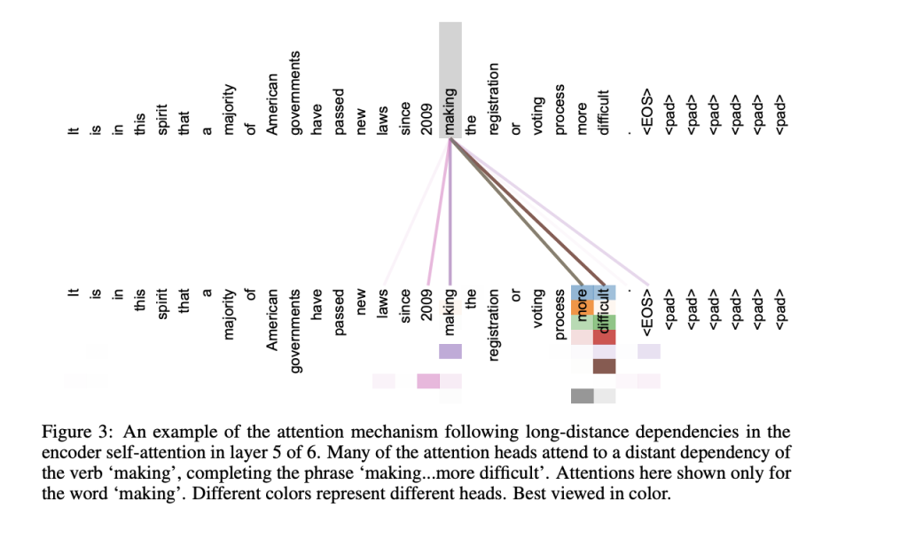
This shows that different heads focus on different parts of the input sequence for every position.

So there’s a faint line between “laws” and “making” and there are more solid lines between “making” and “2009”, “making”, “more” and “difficult”. We can see how this head uses some context around the word “making” instead of connecting it to every position in the sentence.

Some heads might be looking at syntactic relationships, while others might be focusing on semantic ones as this example of anaphora resolution shows:

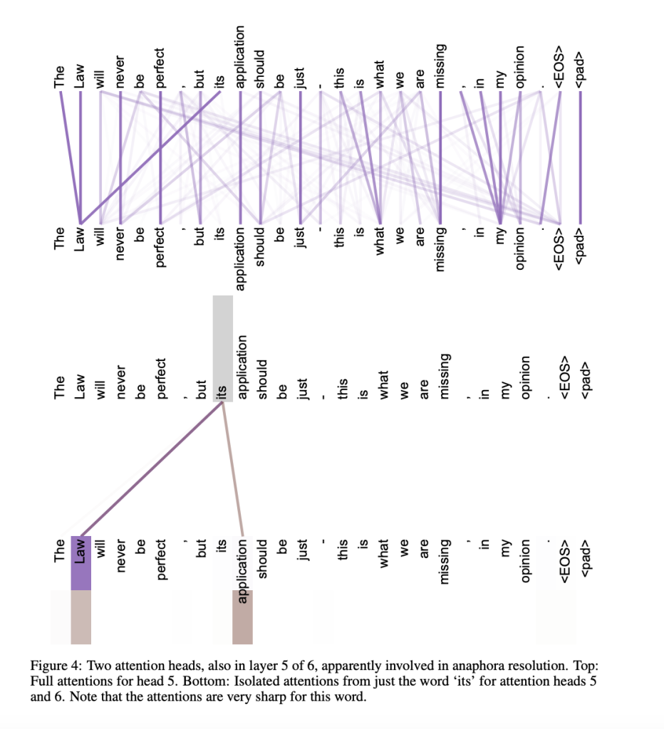
We see that the model determines which entity “its” belongs to by effectively finding “Law” and “application” (Law -> application -> its). In the top part we can see that “opinion” only belongs to “opinion” (itself) and “my”.

The following image shows even more how each head learned to perform a different task

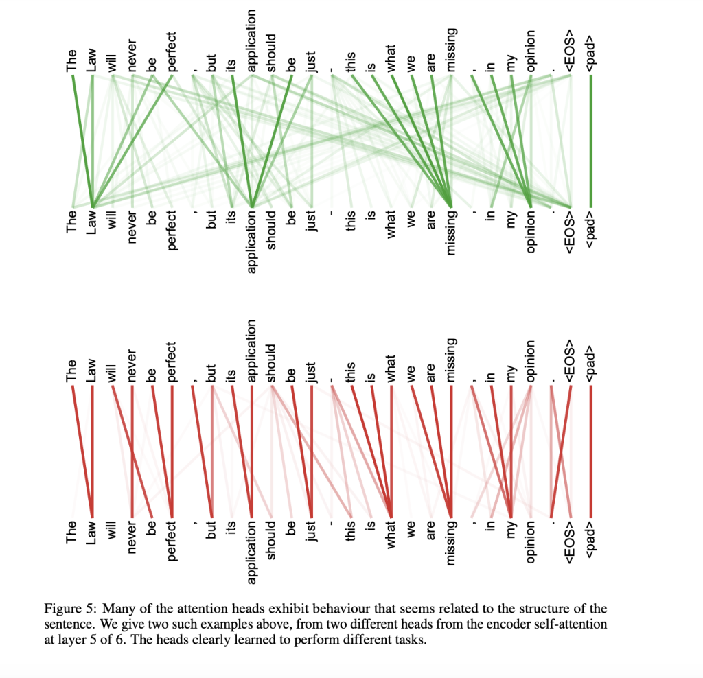
We can notice how the attentions are spread out across the sentence for the green head; each word attends to many others even far from its (like “Law” with “missing”). It’s like a normal distribution with a huge variance. It could be capturing long-range contextual information to understand the meaning of the sentence as a whole. While the attentions for the red head are more focused, like a narrow gaussian distribution. This head could be focusing on local syntactic relationships such as which verb for which subject etc. Or it might be just keeping track of the positional information. Keeping track of fine-grained positional information combined with global contextual information and combined with other syntactic and semantic relationships captured by other heads would make the model completely understand a sentence.

So we can think of the multi-head attention as a mechanism for model to jointly attend to information from different representation subspaces at different positions where each head looks at the input from a different perspective, like looking at some kind of syntactic or semantic relationships.

In an upcoming post where we study the vision transformer, we’re going to see that there is a similar effect happening there as well.

Training Details

Tokenizer:
Byte-pair encoding (BPE)

Tasks:
Machine translation

Datasets:
Standard WMT 2014 English-German (≈$4.5$M sentence pairs, $37k$ tokens in learned vocabulary)
Large WMT 2014 English-French (≈$36$M sentence pairs, $32k$ tokens in learned vocabulary)

Batching:
Sequences of approximate sequence length are batched together
Each batch contains approximately 25k tokens for both source and target sequences

Optimizer:

• Adam: $\beta_{1}=0.9$, $\beta_{2}=0.98$, $\varepsilon=10^{-9}$
• Learning rate: varies according to the following formula with $warmup\_steps=4000$
  $$\frac{1}{\sqrt{d_{model}}}min(\frac{1}{\sqrt{step\_num}},\frac{step\_num}{warmup\_steps^{1.5}})$$
  (we explain more this learning rate here)

Regularization:

• Dropout: all dropout’ rates are $0.1$
  • At the output of each sub-layer
  • After the sum of embedding vectors and positional encodings
• Label smoothing: $\varepsilon_{ls}=0.1$
  • (we explain label smoothing here)

Let’s code the loss function

import torch
import torch.nn as nn
import torch.nn.functional as F

class LabelSmoothing(nn.Module):
    def __init__(self, tgt_vocab_len, smoothing=0.0, padding_index=None):
        super(LabelSmoothing, self).__init__()
        self.n_classes = tgt_vocab_len
        self.smoothing = smoothing
        self.padding_index = padding_index

    def forward(self, logits, target):
        bsz, tgt_seqlen, _ = logits.size()

        # Create smoothed target distribution
        with torch.no_grad():
            target_smoothed = torch.full_like(logits, fill_value=self.smoothing / (self.n_classes - 1))
            target_expanded = target.unsqueeze(2)
            target_smoothed.scatter_(2, target_expanded, 1.0 - self.smoothing)

        # Create a mask to ignore the padding tokens in the target
        if self.padding_index is not None:
            mask = target != self.padding_index
            num_non_padding_tokens = mask.sum()
            mask = mask.unsqueeze(-1).expand_as(logits)
        else:
            num_non_padding_tokens = bsz * tgt_seqlen
            mask = torch.ones_like(logits)

        # Apply log softmax on logits
        log_probs = F.log_softmax(logits, dim=2)

        # Compute the cross-entropy loss over non-padding tokens only
        loss = -torch.sum(log_probs * target_smoothed * mask) / num_non_padding_tokens

        return loss
    
def lr_func(dmodel, step_num, warmup_steps=4000):
  if step_num == 0:
    step_num = 1
  return (dmodel ** (-0.5)) * min(step_num ** (-0.5), step_num * (warmup_steps ** (-1.5)))

def nmt_loss(model_output, ground_truth, labelsmoothing):
   return labelsmoothing(model_output, ground_truth)

We can verify that this loss gives the same results as using PyTorch’s cross-entropy with a label smoothing factor

batch_size = 32
sequence_length = 10
vocabulary_length = 100

logits = torch.randn(batch_size, sequence_length, vocabulary_length)
logits_reshaped = logits.permute(0, 2, 1) # Reshape for Pytorch's inputs
target = torch.randint(1, vocabulary_length, (batch_size, sequence_length))

lsr = LabelSmoothing(100, 0.1)
nn_loss = nn.CrossEntropyLoss(label_smoothing=0.1)

print("Custom Label Smoothing Cross-Entropy Loss:", lsr(logits, target).item())
print("Pytorch Loss:", nn_loss(logits_reshaped, target).item())

We can also check that the masking works correctly

float_value_for_illustration = 123.56

extra_target = torch.full((batch_size, 3), 0, dtype=torch.int64)
target_extended = torch.cat([target, extra_target], dim=1)

extra_logits = torch.full((batch_size, 3, vocabulary_length), float_value_for_illustration)
logits_extended = torch.cat([logits, extra_logits], dim=1)

lsr = LabelSmoothing(100, 0.1, 0)

print("Custom Label Smoothing Cross-Entropy Loss:", lsr(logits_extended, target_extended).item())
print("Pytorch Loss:", nn_loss(logits_reshaped, target).item())

As for the learning rate we use the LambdaLR class

from torch.optim import Adam
from torch.optim.lr_scheduler import LambdaLR

optimizer = torch.optim.Adam(model.parameters(),
                             lr=1.0,
                             betas=(0.9, 0.98),
                             eps=1e-9
                             )
lr_scheduler = LambdaLR(optimizer=optimizer,
                        lr_lambda=lambda step: lr_func(d_model, step)
                        )

Some “Why” and “How” Questions

Why do we need the keys?

As explained here, the keys allow us to relate an element in a sequence to all others and help weigh their relevance with regard to the query and the values.

Why the queries and keys have the same dimensions?

It’s required to perform the attention computation, as you can see here.

Why h heads instead of one?

As discussed here, having $h$ heads allows the model to capture different aspects of data, hence increasing its representation power. We can look at the different heads like having many kernels in the convolution steps of a convolutional neural network (CNN), it introduces some flexibility in learning different concepts and relationships in the data.

Why *scaled* dot-product attention?

Scaling the dot-product allows us to have better gradients. As explained here, not scaling the dot-product leads to high values inside of the softmax which pushes it to regions where it’s almost constant and its gradients almost zero. This issue only happen for higher values of $d_{k}$.

Why don’t we mask the padding tokens in the queries?

We don’t mask the padding tokens’ positions in the queries (which results in $-\infty$ rows in the padding masks) because it’s important to know where the padding tokens are. That’s why we don’t mask them in the queries but we mask them in the keys to nullify their contribution in the attention of non-padding tokens.

Why the weights of the two embedding layers and the pre-softmax linear layer are shared?

It’s because it helps improve performance. See this paragraph or read this paper.

Why do we scale the tokens’ embeddings by $\sqrt{d_{model}}$?

There’s no clear answer as to why this is done but some hypotheses are mentioned here. The hypotheses are that it’s not actually needed, or that it’s used to initially make the embeddings bigger than the positional encoding or that it’s used because we’re sharing the weights as mentioned before.

Why do we need positional encoding?

It’s because the Transformer doesn’t have an inherent understanding on order in the sequences since the attention mechanism and the feed-forward networks process the positions in parallel. It would be less the case if it contained convolutions and recurrence as the author states. We discuss this more here.

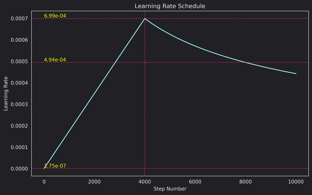
Why that specific learning rate and how it works?

The learning rate increases linearly for exactly $warmup\_steps$ then decreases in the same fashion as $x\mapsto \frac{1}{\sqrt{x}}$, both these variations are scaled with $\frac{1}{\sqrt{d_{model}}}$.

I think the exact formula is the result for many experiments but some main points are:

We want to scale down the learning rate the higher the model dimension, thus the scaling by $\frac{1}{\sqrt{d_{model}}}$. High dimension spaces are more complex to navigate so we want a smaller learning rate to make precise updates.

In the early stage of training, a small learning rate is inefficient and a large learning rate can cause divergence, so we want to slowly increase the linear rate to explore the optimization landscape and escape local minimas.

As the model is converging, we slowly decrease the learning rate. The square root decay being a less aggressive decay than an exponential decay, it might be a good choice to slowly transition from the learning rate increase phase to the convergence phase.

$\frac{1}{\sqrt{step\_num}} = \frac{step\_num}{warmup\_steps^{1.5}}$ leads to $warmup\_steps^{1.5} = step\_num^{1.5}$. So the cutoff between the linear increase and the inverse square root decay is exactly $warmup\_steps$.

Now if $step\_num < warmup\_steps$ then $\frac{1}{step\_num^{1.5}} > \frac{1}{warmup\_steps^{1.5}}$ which leads to $min(\frac{1}{\sqrt{step\_num}},\frac{step\_num}{warmup\_steps^{1.5}}) = \frac{1}{warmup\_steps^{1.5}}$ so before the first $warmup\_steps$ we’re effectively increasing linearly the learning rate. Below is a graph that shows the evolution of the learning rate as a function of the steps for $d_{model}=512$

What is label smoothing and why is it used?

Label smoothing is introduced in the paper Rethinking the Inception Architecture for Computer Vision as a regularization method which is applied to the cross-entropy loss. Generally in classification settings, we use a hard target distribution (one-hot encoding of the labels) in our cross-entropy loss. With label smoothing, we use a softer distribution, instead of having $1$ for the correct label and $0$ for the other labels, we use $1-\varepsilon$ for the correct label and $\varepsilon$ for the others, where $\varepsilon$ is the smoothing parameter.

That’s all label smoothing is, instead of using that hard distribution in your cross-entropy, use this distribution instead. This is what most implementations do anyways, but one can make different softer target distributions. If your original target distribution is $q(k|x)$, then the softer version of it is $q'(k|x) = (1-\varepsilon )q(k|x)+\varepsilon u(k)$ where $u(k)$ is a distribution over the labels independent from $x$, your training example.

In the case of a hard target distribution we have $q(k|x)=\delta_{k,y}$, the Kronecker delta, where $\delta_{k,y}=1$ if and only if $k = y$, otherwise it’s equal to $0$, then $q'(k|x)= (1−\varepsilon )\delta_{k,y} + \varepsilon u(k)$.
And if on top of that you chose $u(k)$ to be the uniform prior distribution over the labels then $q'(k|x) = (1 - \varepsilon)\delta_{k,y} + \frac{\varepsilon}{K}$ where $K$ is the number of classes, in our case, the length of our vocabulary.

So why one would use label smoothing and how does it act as a regularization method?

The traditional setting of classification, we have an example $x$ and the model computes the probability of each class $k \in \{1 . . . K\}: p(k|x) = \frac{exp(z_{k})}{\sum_{i=1}^{K}exp(z_{i})}$ at the softmax level, where $z_{i}$ are the logits. Then we compute the cross-entropy loss $l = - \sum_{k=1}^{K}log(p(k|x))q(k|x)$.

When we minimize this loss, it’s equivalent to maximizing the expected log-likelihood of a label where the label is selected according to the ground-truth distribution. In the usual case of classification this ground-truth distribution is the hard distribution $q(k|x)=\delta_{k,y}$ where $y$ is the correct label for $x$. (We omit the mention of $x$ in the $\delta$ for clarity). Our predictions are correct if and only if $p(y|x)=1$ (the probability prediction of our model for label $y$ is $1$), looking at the softmax formula $p(y|x) = \frac{exp(z_{y})}{\sum_{i=1}^{K}exp(z_{i})}$ this can happen only for $z_{y} \rightarrow +\infty$, which can’t happen in purpose. But we get a good approximation if $z_{y}$ is very large compared to $z_{k}$ for $k \neq y$. When that happens, this causes two main issues:

1. Overfitting: When $z_{y}$ is very large compared to $z_{k}$ then the model becomes too confident in its prediction about the training data leading it to memorize particularities of the training set which hinders its ability to generalize to unseen data.
2. Reduced model adaptability: when we minimize the cross-entropy loss, we compute its gradients according to the logits (the activations of the neurons before applying the softmax) which are $\frac{\partial l}{\partial z_{k}} = p(k)−q(k)$. So when the correct logit $z_{y}$ is too large, this leads to $p(k)$ to be very close to $1 = q(k)$, and the same for $k \neq y$ $p(k)$ is almost $0 = q(k)$. So the gradients get very small. This is a huge issue during the early training of the model since the very small updates won’t be enough for it to learn appropriately from all the variety in the training set.

When we minimize this loss we compute its gradients according to the logits (the activations of the neurons before applying the softmax) which are $\frac{\partial l}{\partial z_{i}} = p(k)−q(k)$.

But now, replace $q$ with $q'$, the gradients become $\frac{\partial l}{\partial z_{k}} = p(k)−q'(k)$ and in the case of $q'(k|x) = (1 - \varepsilon)\delta_{k,y} + \frac{\varepsilon}{K}$ we have $\frac{\partial l}{\partial z_{k}} = p(k)−(1- \varepsilon)q(k)-\frac{\varepsilon}{K}$ so even if $p(y)$ becomes $q(y)$ and $p(k)$ becomes $0$ for $k\neq y$ we get $\frac{\partial l}{\partial z_{y}} = \frac{(K-1)\varepsilon}{K}$ and $\frac{\partial l}{\partial z_{k}} = \frac{\varepsilon}{K}$. So the gradients never become too small. So, label smoothing does solve the issues mentioned above.

You can intuitively see its regularization effect since the model is no longer trained to push the logit for the correct class $z_{y}$ too large compared to the other logits since now it has to predict a probability of $1-\varepsilon$ and spread $\varepsilon$ across the other logits. It’s learning a slightly uncertain distribution where the correct class doesn’t have a probability of $1$ so the model has to be cautious.

But we can also see it theoretically, let’s denote the cross-entropy loss by $H$, then

The second loss penalizes the deviation of predicted label distribution $p$ from the prior $u$, with the relative weight $\frac{\varepsilon}{1-\varepsilon}$. In the paper the authors also mention that this deviation can be captured by the KL-divergence.

Helpful Links

Unfortunately I can’t trace back all of the https://ai.stackexchange.com/ posts that I’ve read and helped me understand this topic better. But it’s definitely a trove of knowledge.
Yannic Kilcher’s video about this paper also helped me clarify some points.
Though no particular source inspired me for the from-scratch implementation of the architecture, I did come across The Annotated Transformer from Harvard NLP which is a better implementation than mine, with distributed training. I also did come across this blog post, from the user pi-tau on the AI Stackexchange. Some of the answers from that user are really good and helped me clarify some points in my mind.