On this page
After publishing my first translation article and discussing it on Reddit, two suggestions appeared repeatedly in the replies:
- use a model trained specifically for translation;
- constrain the response through structured decoding and a JSON Schema.
Publication note. While preparing the public experiment artifacts, I found two evidence-retention limits in the historical chunk curve from the first article. In 360 source–model–language–chunk conditions, 7,056 table-cell translations were generated and inserted into the final documents, but the historical runner did not retain them as separate request outputs. It stored only the prose pairs intended for COMET-QE. These are repeated experimental conditions over the 340 unique source texts, not 360 additional sources. This is an instrumentation limitation, not model failure: the assembled translations used in the analysis were retained, but those 360 condition rows cannot be reconstructed solely from the published unit rows.
In another 49 conditions, 51 prose requests genuinely returned empty cleaned outputs. All came from Gemma 3, mostly at chunk labels 4,096 and 8,192. The historical runner recorded the empty-unit counts, and the omissions are present in the assembled documents, but it did not retain a complete raw API record for every request. The public data therefore represents those known processed outputs explicitly as empty strings while leaving the unavailable raw-response fields null.
Context entered the study for a different reason. While designing the structured-output experiment, I had to decide whether one request should translate a single unit or pack several consecutive units into one response. That brought me back to earlier experiments in which previous source and translation pairs were shown to the model to preserve coherence. When I reviewed those experiments, I found that their comparisons were not rigorous enough to support the conclusions I wanted to reuse. I therefore reran the context comparison before testing specialists and structured outputs.
The follow-up therefore asks three related questions: whether previous translation pairs help as context, whether a translation specialist improves on the selected baseline, and whether structured outputs make the interface safer. These interventions operate at different layers of the system. Previous pairs change the prompt context. A specialist changes the model, its interface, and sometimes its decoding policy. A schema constrains which output-token sequences the decoder can emit. Those mechanisms address only part of the acceptance contract: none automatically protects code or establishes that the returned text is a complete translation.
I tested the interventions separately. Combining them immediately would have produced a new pipeline, but it would not have told me which intervention helped, which one hurt, or whether one change merely concealed the failure caused by another.
The baseline throughout this follow-up is the system selected in the first study: the FP8 Gemma 4 checkpoint with the structure-aware method at chunk label 512. The label corresponds to approximately 2,048 source characters in this splitter. It is not a claim that every translation unit contains 512 model tokens.
I will call the baseline method P0. P0 parses one source document into typed regions, keeps recognized code and mathematics under Python control, translates prose in bounded units, translates table cells separately, and reconstructs the document deterministically. Each prose unit is translated independently. The exact public checkpoint is a local snapshot of RedHatAI/gemma-4-31B-it-FP8-dynamic, served with vLLM 0.22.1 and Transformers 5.6.0 on one H100 64 GB GPU.
Here, a cleaned translation is the model’s raw prose output after deterministic cleanup removes an accidental enclosing Markdown fence and surrounding whitespace. It is not corrected, selected, or manually edited.
Two comparison labels also appear throughout the article. Pc keeps P0’s parsing, unit boundaries, and reconstruction, but adds up to three preceding source and cleaned translation pairs as context before the same current translation unit. RAW is the parser-free comparison: it divides the source into bounded chunks without recognizing code, mathematics, tables, or reasoning wrappers, exposes every character to the model, and concatenates the generated chunks in order. Their full implementations are described in the corresponding experiment sections.
The structured experiment also distinguishes two interfaces. In prompt-only JSON, the prompt requests a JSON object but decoding remains unconstrained. In schema-constrained decoding, the same response is registered with a JSON Schema that vLLM uses to restrict ordinary content tokens to sequences compatible with the required object.
The question is not whether context, specialists, or schemas can ever help translation. The experiments ask whether these particular interventions improve this qualified baseline on the same reasoning-data population.
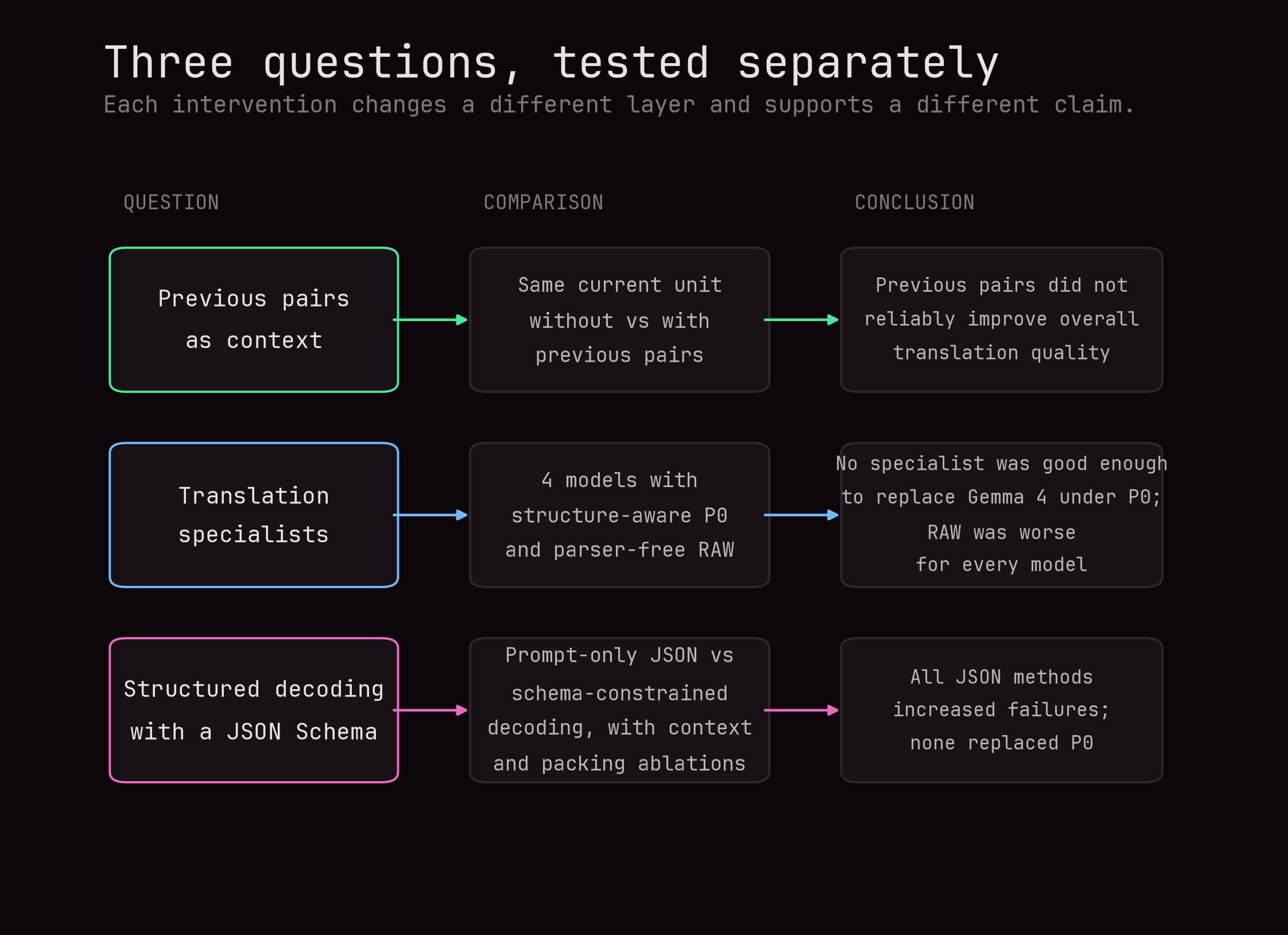
Qwen3.8-27B was released after I designed that three-question study. I added it later as a matched general-model substitution, not as a fourth suggestion and not as another translation specialist. That distinction is why it does not appear in FIG_01.
Repeating the context experiment properly
The first study contained several context variants, but they were not clean enough to settle the context question.
I reran the comparison from fresh requests. The paired experiment used the same 340 source rows, six target languages, P0 parser, unit boundaries, translation instruction, cleanup, and reconstruction in both arms:
- P0 saw only the current source unit and generated its translation.
- Pc saw up to the three immediately preceding source and cleaned translation pairs as ordinary chat history, followed by the same current source unit. It generated only the current translation.
Pc processed each document sequentially because the translation of unit $i$ became part of the context for unit $i+1$. P0 could process a document’s independent units concurrently. Previous context crossed prose blocks and the pre-reasoning, reasoning, and post-reasoning regions. Table cells remained independent because a cell’s preceding neighbor is often a layout neighbor rather than a useful discourse predecessor. More honestly, I did not think a separate table-history policy was worth the additional parser and prompt work for this comparison. Table cells received the same treatment in both arms, which preserves the P0–Pc comparison for the intervention actually tested, although it leaves open whether table-aware context would help tables. Recognized code and mathematics never entered either model as translatable text.
A simplified Pc request for the third prose unit looked like this:
user:      [translation instruction + source unit 1]
assistant: [cleaned translation 1]
user:      [translation instruction + source unit 2]
assistant: [cleaned translation 2]
user:      [translation instruction + source unit 3]
assistant: ?
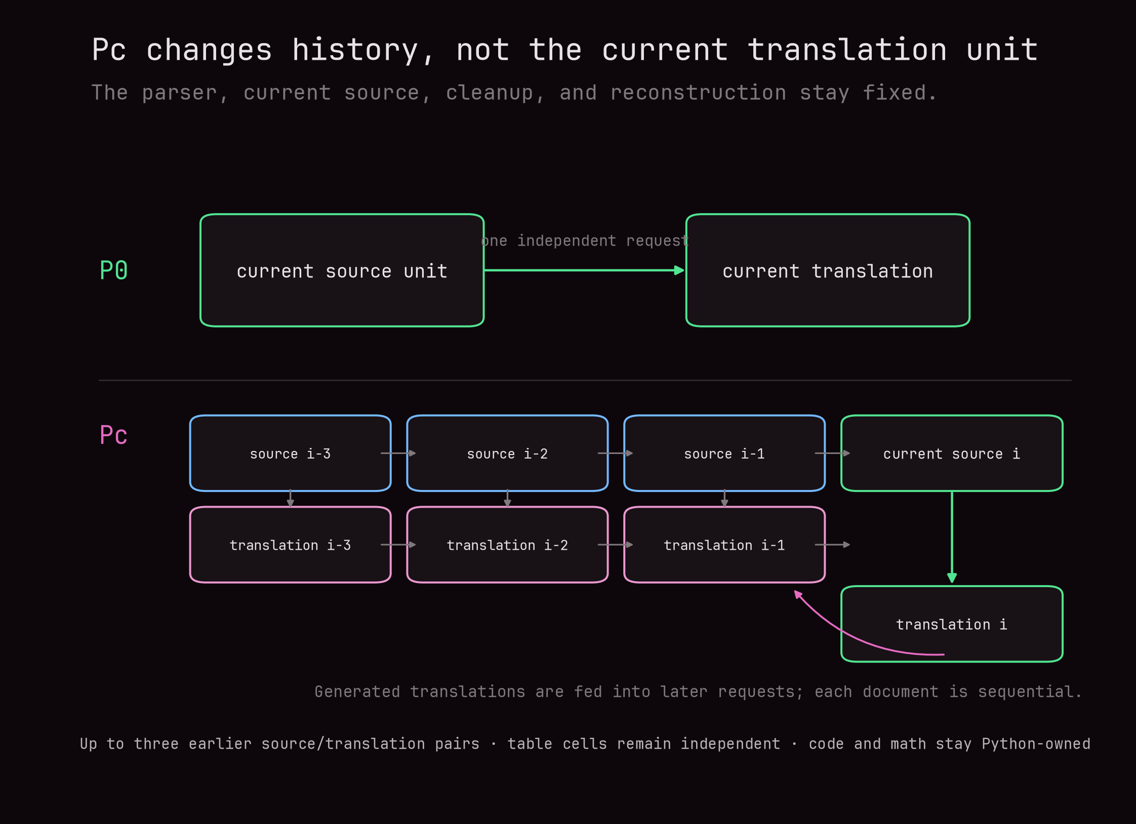
The current source in the final user turn was byte-identical to the corresponding P0 source unit. Pc did not ask the model to revise earlier translations. Those earlier pairs were read-only evidence for terminology and continuity, although they could still influence the current output.
This design tests one concrete form of context.
The populations and paired statistic
All 340 sources were retained for operational checks. Three rows with source-side contamination known before this comparison were excluded from quality scoring, leaving 337 sources and $337 \times 6 = 2{,}022$ source-language pairs.
Not every source had a later prose unit that could receive prior context. Of the 337 sources retained for quality scoring, 234 had at least one such unit. Each was translated into six languages, so the context-eligible population contains $234 \times 6 = 1{,}404$ source-language pairs. The complete scoring population answers how the deployable systems compare over all retained sources. The context-eligible population asks the narrower question on sources where Pc could actually differ from P0.
For source document $d$ and target language $\ell$, the paired document-quality difference is $\Delta_{d,\ell}=Q_{d,\ell}^{Pc}-Q_{d,\ell}^{P0}$.
$Q$ is the document aggregate from the same reference-free wmt22-cometkiwi-da pipeline described in the first article.
Positive $\Delta$ favors Pc. Confidence intervals use 10,000 source-cluster bootstrap repetitions with seed 20260725. Each repetition samples source IDs with replacement. When it selects one source, it includes that source’s six separate language comparisons and all the evaluation units used to construct those document scores. If a source is sampled twice, the complete group appears twice. Keeping the group intact preserves correlation among translations of the same reasoning trace instead of treating the 2,022 source–language pairs as independent observations.
The analysis also reports two different tail measurements:
- the worst-unit COMET score is the minimum scoring-unit value inside a document;
- the severe composite marks a source-language document when at least one translation unit ends by length, is empty, strongly reverts to English, emits a new code fence, expands or contracts severely, develops excessive repetition, or produces an abnormal invisible or formatting-character run.
The severe composite is an operational alarm assembled from pre-existing tripwires. One document can trigger it through several mechanisms.
Context produced a trade rather than a win
Across the complete 337-source quality population, mean document COMET changed from 0.783225 for P0 to 0.782438 for Pc. The paired difference was -0.000787, with a 95% source-cluster interval of [-0.001295, -0.000299].
The effect was small, but it was not a hidden gain canceled only by documents without context. On the 234-source context-eligible population, the mean difference was slightly more negative:
| Measurement | P0 | Pc | Pc − P0 | 95% source-cluster interval |
|---|---|---|---|---|
| Document COMET, 1,404 context-eligible source-language pairs | 0.768671 | 0.767480 | −0.001191 | [−0.001906, −0.000522] |
| Worst-unit COMET, same 1,404 pairs | 0.635866 | 0.637831 | +0.001965 | [−0.001729, +0.006047] |
| Severe composite rate, same 1,404 pairs | 87/1,404 (6.20%) | 63/1,404 (4.49%) | −1.71 percentage points | [−3.63, +0.14] pp |
The six languages are not collapsed into one score for a source. Each source contributes six separate source–language documents. Let $q_{d,\ell,u}^{m}$ be the COMET-QE score of evaluation unit $u$ for source $d$, target language $\ell$, and method $m \in \{P0,Pc\}$. Within one fixed source–language translation, the document value is the combined-token-length-weighted aggregate $Q_{d,\ell}^{m}=\sum_u w_uq_u/\sum_u w_u$, where $w_u$ is the combined source-and-candidate content-token count measured with the evaluator’s InfoXLM tokenizer. The table averages the 234 document values within each language and then averages the six language means. Because every language has exactly 234 sources, this is numerically equal to averaging all 1,404 source–language document values together.
Worst-unit COMET changes only the within-document operation. For each source–language translation, it keeps the lowest scoring evaluation unit, $W_{d,\ell}^{m}=\min_u q_{d,\ell,u}^{m}$, and then averages those document-level minima in the same way. The procedure does not select the worst language for a source. One source contributes six separate minima, one per target language.
The severe composite is binary at the same source–language-document level: $S_{d,\ell}^{m}=1$ when at least one translation unit triggers a severe tripwire and $0$ otherwise. A source can therefore contribute between zero and six flagged translations. P0 triggered the composite in 87 of the 1,404 source–language documents, while Pc triggered it in 63. Those counts give 6.20% and 4.49%; their difference is −1.71 percentage points. The confidence intervals for all three rows still resample source IDs and keep the six language outcomes for each source together.
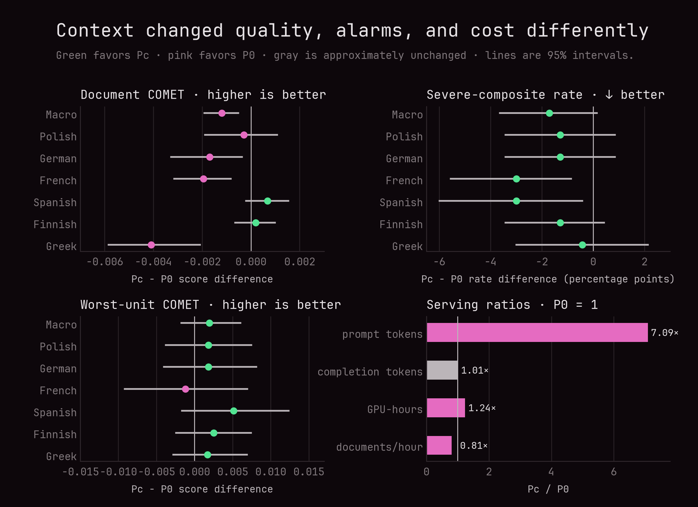
Mean document COMET favors P0: Pc scored 0.001191 lower on the 1,404 context-eligible source–language documents, and the interval [-0.001906, −0.000522] lies entirely below zero. Worst-unit COMET points in the other direction: Pc’s mean document minimum was 0.001965 higher. Its interval [-0.001729, +0.006047] crosses zero, however, so this result remains compatible with a small Pc gain, no difference, or a small loss.
Pc also had a lower observed severe-composite rate in every language. The six-language point estimate was −1.71 percentage points, but its interval [-3.63, +0.14] crosses zero. Zero represents equal severe-composite rates, so the macro result remains compatible with a Pc reduction, no difference, or a very small increase. The fact that all six observed differences are below zero is suggestive, but the number of alarms is small enough that the per-language estimates remain uncertain.
French had an interval of [-5.56, −0.85] percentage points and Spanish [-5.98, −0.43]. These are the only two language intervals that lie entirely below zero. Because the difference is Pc minus P0 and a lower severe rate is better, they provide evidence of a reduction for French and Spanish. The intervals for Polish, German, Finnish, and Greek cross zero, as does the six-language interval, so the experiment does not establish a general reduction across languages.
Language heterogeneity matters. The all-quality document-COMET changes were:
| Target language | Pc − P0 document COMET | 95% source-cluster interval | Documents materially favoring Pc / within ±0.01 / favoring P0 |
|---|---|---|---|
| Polish | −0.000042 | [−0.001209, +0.000998] | 21 / 297 / 19 |
| German | −0.001144 | [−0.002301, −0.000157] | 15 / 298 / 24 |
| French | −0.001120 | [−0.002020, −0.000313] | 11 / 299 / 27 |
| Spanish | +0.000682 | [+0.000016, +0.001342] | 18 / 310 / 9 |
| Finnish | −0.000119 | [−0.000822, +0.000536] | 9 / 315 / 13 |
| Greek | −0.002980 | [−0.004254, −0.001547] | 16 / 262 / 59 |
“Materially” uses an absolute document-COMET difference greater than 0.01. That band was fixed for this analysis as a practical sorting rule.
Greek accounts for much of the negative macro result. Spanish moves slightly in the other direction. A single pooled number would conceal both facts.
The two methods are nevertheless extremely close on mean COMET. This automatic evaluation cannot settle subtler questions such as whether context improves terminology, pronoun resolution, or discourse continuity while causing different local omissions. That would require a finer evaluation: a blinded rubric designed around those phenomena, followed by native-speaker labels on a calibrated subset. I defer that comparison because the context ablation is not the central experiment in this follow-up. The evidence here supports no demonstrated quality gain from Pc, not the stronger claim that P0 is linguistically better in every respect.
One case where context helped, and one paired regression
The paired packet makes the trade less abstract. One French source was a programming problem about reconstructing a damaged binary arithmetic expression. A period represented an unreadable character, and the objective was to fill the damaged expression so that its value was as large as possible. For example, 0.0 can become the binary number 010, whose decimal value is 2, while ... can become 111, whose value is 7.
The parser placed the problem statement and its sample cases in consecutive prose units. Pc’s history contained the entire preceding source unit as a user turn and its generated French translation as an assistant turn. The exact final portion of that history pair was:
Previous source turn:
Input

The input consists of one line and is given one formula to decipher.
The formula is 1 to 100 characters. Up to 5 characters cannot be read
for one formula and are represented by ".". The characters contained
in the given formula are either 01 +-* ().

Output

Find the one that maximizes the calculation result among the original
formulas, and output the calculation result in decimal notation.
Output -1 if you can't make what you think is the original formula
no matter how you fill in the unreadable characters.
Previous assistant turn:
Entrée

L'entrée consiste en une seule ligne et donne une formule à déchiffrer.
La formule fait de 1 à 100 caractères. Jusqu'à 5 caractères ne peuvent
pas être lus pour une formule et sont représentés par ".". Les caractères
contenus dans la formule donnée sont soit 01 +-* ().

Sortie

Trouvez celle qui maximise le résultat du calcul parmi les formules
originales, et affichez le résultat du calcul en notation décimale.
Affichez -1 si vous ne pouvez pas reconstituer ce que vous pensez être
la formule originale, quelle que soit la manière dont vous remplissez
les caractères illisibles.
The next source unit was:
Examples

Input

000

Output

0

Input

0.0

Output

2

...
P0 saw only that unit and returned:
Veuillez fournir le texte que vous souhaitez faire traduire.
Pc had the preceding translated problem statement in its history and returned:
Exemples

Entrée

000

Sortie

0

Entrée

0.0

Sortie

2

...
This is the kind of case context should repair. The current unit looks like an isolated interaction fragment to P0, while the previous pair tells Pc that it is the examples section of the same document. Its unit-level COMET difference was +0.400995.
That was the case where context helped. The reverse also occurred in a French translation of a long reasoning trace about implementing 32-bit bitwise operations in dc. The source writes its name inconsistently as DC, but dc is a stack-based, reverse-Polish arbitrary-precision calculator that can also execute macros. Its syntax is intentionally terse: numbers are pushed onto a stack, arithmetic operators consume values from that stack, registers store intermediate values, and bracketed strings can act as recursively invoked programs.
Pc received the three immediately preceding source and translation pairs. The source itself was already a noisy mixture of English, Chinese, Korean, and symbols. In the Pc history, the first translation failed the strict literal-preservation diagnostic, although it did not enter the severe composite. The second triggered the severe English-reversion alarm because it left much of the natural language untranslated. The third was short and clean.
The matched P0 outputs are important here. P0 translated the same three source units independently, without history. On the first unit, P0 translated more of the Chinese fragments into French, although both P0 and Pc failed the strict literal-preservation check. On the second, P0 translated the mixed-language source much more completely and remained outside the severe composite, while Pc retained long stretches of English and Chinese. The third output was byte-identical in both arms. These are exact excerpts; the ellipses mark text omitted from the article:
History pair 1
source:  交换a和 1 ... 交换两次得到 [1-b, a]
P0:      échanger a et 1 ... échanger deux fois pour obtenir [1-b, a]
Pc:      交换a和 1 ... 交换两次得到 [1-b, a]

History pair 2
source:  这可以 be done通过 the steps ...
P0:      Cela peut être fait via les étapes ...
Pc:      Cela peut be done通过 the steps ...

History pair 3
source:  Testing the functions:
P0:      Test des fonctions :
Pc:      Test des fonctions :
The current source requires an important correction. It was malformed before translation: it contained one <think> opener and two </think> closers. The parser extracted the first balanced <think>…</think> region, kept those two recognized wrapper tags out of the model requests, and reinserted them during reconstruction. Everything after that first closing tag became post-reasoning content.
The second </think> had no matching opener. The parser did not recognize it as a wrapper and left it inside an ordinary post-reasoning prose unit. The current unit therefore did not cross a parser-controlled reasoning boundary. Its exact model-visible content contained an orphan closing tag followed by the final answer:
However, DC does not Support directly using 'b (binary)' notation,
so the test cases use decimal representations.

Note: The above code may have syntaxical errors ...

</think>

To solve this problem, we need to implement bitwise AND, OR, XOR,
and NOT functions ...

### Approach
...

### Solution Code
...
P0 had no preceding pairs. It translated the note, continued past the orphan closing tag, and translated the approach and solution code:
Cependant, DC ne supporte pas directement l'utilisation de la notation
'b (binaire)', donc les cas de test utilisent des représentations décimales.

Note : Le code ci-dessus peut contenir des erreurs syntaxiques ...

Pour résoudre ce problème, nous devons implémenter les fonctions bitwise
AND, OR, XOR et NOT ...

### Approche
...

### Code de la Solution
...
Pc translated only the material before the boundary:
Cependant, DC ne supporte pas directement l'utilisation de la notation
'b (binaire)', donc les cas de test utilisent des représentations décimales.

Note : Le code ci-dessus peut contenir des erreurs syntaxiques ...
L'implémentation réelle pourrait nécessiter d'ajuster soigneusement les
sauvegardes de registres et les opérations d'empilement.
Both requests received this same malformed current unit and recorded finish_reason=stop; this was not an output-token limit. P0 generated 882 completion tokens and Pc generated 163. The Pc output therefore lost the final answer even though its request completed normally. The unit’s COMET difference was −0.041805, and the case triggered the severe undertranslation alarm.
This is an observed paired regression in the Pc condition, not a clean context-only example. Pc consumed one history pair with a strict-diagnostic failure, one with a severe English-reversion failure, and one clean pair, then chose a different completion boundary from P0 on the same malformed current source unit. The evidence cannot separate the history effect from its interaction with the orphan tag, nor identify one history fragment as the cause.
These are frozen review cases, not representative rates. The first shows the intended contextual mechanism directly. The second exposes a narrower interaction among generated history, an orphan structural tag, and the model’s stopping decision. It should not be generalized into a claim that clean translation history causes omissions.
Did a bad previous translation contaminate the next one?
Pc feeds generated translations back into later requests, so error propagation is an obvious concern. The retained unit sequence lets us ask whether a current Pc-only severe failure follows a previous Pc unit already marked severe. A Pc-only severe failure means that the current Pc output enters the severe composite while the matched P0 output for that same current source unit does not.
Lag describes position, not the number of pairs in the prompt. For current prose unit \(i\), lag one inspects Pc unit \(i-1\), lag two inspects \(i-2\), and lag three inspects \(i-3\). The 37,926 lag-one-eligible current units are therefore all later prose units with an immediate predecessor across the six languages. Of those, 1,404 had one available history pair, 1,308 had two, and 35,214 had the maximum of three. The denominator does not mean that every unit had exactly one pair in context.
Among the 77 current units whose lag-one Pc predecessor was severe, 67 were severe in neither arm, 9 were severe in both arms, 1 was severe only under P0, and 0 were severe only under Pc.
At lag two, 69 current units had a severe Pc unit two positions earlier. Four of their current outputs were severe only under Pc. This does not mean that those prompts contained two severe history pairs. Only nine current units had severe Pc predecessors at both lag one and lag two. The other 60 lag-two cases had a non-severe immediate predecessor. The dc case above is one of the four lag-two Pc-only failures: unit 23 had severe English reversion, unit 24 was clean, and unit 25 was severe under Pc but not P0.
For every current unit at a chosen lag, the analysis records two separate variables:
- A history-group label, determined only by the earlier Pc unit. The current unit enters the severe-history group if Pc unit \(i-k\) was severe at lag \(k\), and the clean-history group otherwise.
- A current paired outcome, determined only by the two outputs for current unit \(i\):
+1if Pc is severe and P0 is not,0if both arms have the same severe status, and−1if P0 is severe and Pc is not.
The history label decides which group contains the current unit. The number being averaged is always the current paired outcome. Within one source ID, the analysis averages those outcomes in the severe-history group, separately averages them in the clean-history group, and subtracts:
source-level propagation comparison
= mean current paired outcome in the severe-history group
− mean current paired outcome in the clean-history group
A positive result means that Pc developed more current severe failures relative to P0 after a severe item appeared in its history. Zero means that the relative Pc-versus-P0 failure rate did not change. A negative result means that Pc had fewer relative failures after severe history.
The conversion from counts to percentage points follows directly from the paired outcome. Let \(S_i^{Pc}\) equal 1 when the current Pc output is severe and 0 otherwise, and define \(S_i^{P0}\) in the same way. The paired outcome for current unit \(i\) is:
\[ Y_i = S_i^{Pc} - S_i^{P0}. \]For either history group \(G\), averaging those outcomes gives:
\[ \bar{Y}_G = \frac{1}{n_G}\sum_{i \in G}\left(S_i^{Pc}-S_i^{P0}\right). \]Because a sum of binary indicators is a count, the same mean can be written as:
\[ \bar{Y}_G = \frac{N_{\text{Pc severe},G}}{n_G} - \frac{N_{\text{P0 severe},G}}{n_G}. \]After canceling units that are severe in both arms, this is also:
\[ \bar{Y}_G = \frac{N_{\text{Pc-only severe},G} - N_{\text{P0-only severe},G}}{n_G}. \]The second line is Pc’s severe rate minus P0’s severe rate in that history group. Units severe in both arms appear once in each count and cancel, while units severe in neither appear in neither count.
For a concrete example, suppose one source ID contributes 100 current units to the severe-history group. Fifteen are severe only under Pc, 5 only under P0, 10 under both, and 70 under neither. Pc is therefore severe on \(15+10=25\) units and P0 on \(5+10=15\):
\[ \bar{Y}_{\text{severe history}} = \frac{25}{100}-\frac{15}{100} = \frac{15-5}{100} = 0.10. \]The value \(0.10\) is a difference between proportions. Multiplying by 100 expresses it as a 10-percentage-point difference. If the clean-history group has \(\bar{Y}_{\text{clean history}}=0.02\), that is a 2-percentage-point difference. The source-level propagation comparison is then:
\[ 0.10-0.02=0.08, \]or 8 percentage points. This is not an 8 percent relative increase. A relative percentage would require dividing by a chosen baseline rate, which this comparison does not do.
This within-source subtraction requires current units in both history groups. A source ID containing only clean prior units, or only severe prior units, cannot contribute because one group mean is missing. That leaves 23 source IDs at lag one, 21 at lag two, and 19 at lag three.
At lag two, the mean propagation comparison across the 21 contributing source IDs was +3.10 percentage points. To show its uncertainty, I resampled those source IDs with replacement 10,000 times and recomputed the mean. The middle 95 percent of those bootstrap means ran from −12.84 to +19.85 percentage points. The negative end corresponds to fewer relative Pc failures after severe history, zero corresponds to no change, and the positive end corresponds to more. The interval covers all three, so the sample does not determine the direction of the association. It also remains observational: difficult source material can cause both a severe prior translation and a severe current translation without the first failure causing the second.
This does not establish that propagation is absent. It says the representative sample contains too few source IDs with current units in both history groups to estimate it precisely. The fixed review packet includes the observed sequences rather than turning a sparse result into a safety claim.
Temperature zero did not make the control outputs identical
The first prose unit of a document has no previous context. Its P0 and Pc visible messages are identical. Those requests provide a useful control for execution drift outside the intended context intervention.
Depending on language, only 26.1% to 50.1% of processed first-unit outputs were byte-identical across the two independent runs. Identical table-cell requests were much more stable, with 98.0% to 100% identical outputs. The model was sampled at temperature zero with the same request seed, but different scheduling and batching still produced output variation.
The first-unit requests contain no translation history, so any Pc-minus-P0 COMET difference there cannot be attributed to context. I used that observed difference as a baseline for a sensitivity check. For each of the 1,404 context-eligible source-language documents, I first computed the mean Pc-minus-P0 COMET difference across all later, context-exposed prose units. I then subtracted the Pc-minus-P0 COMET difference of that document’s first prose unit:
adjusted comparison
= mean of later-unit (Pc − P0) COMET differences
− first-unit (Pc − P0) COMET difference
The subtraction asks whether the later units moved further toward Pc or P0 than the difference already observed when both methods received an identical first-unit prompt. A positive value favors Pc after this adjustment, a negative value favors P0, and zero means no additional shift.
Across all six languages, the mean first-unit difference was +0.000165, while the mean of the per-document later-unit differences was −0.000033. Their difference was therefore −0.000198. Each source ID kept its six languages together during bootstrap resampling, producing a 95 percent interval of [-0.002101, +0.002699].
Keeping those six comparisons together matters because they are translations of the same reasoning trace, not six independent source documents. They share the same subject, length, structure, instructions, code, mathematics, and source-side defects. A difficult trace can therefore affect several target languages at once. Resampling the 1,404 source-language documents independently would count those correlated outcomes as separate evidence and could make the uncertainty interval artificially narrow. The source-cluster bootstrap instead samples one of the 234 source IDs and carries all six language comparisons with it. This preserves their correlation, keeps the six-language balance intact, and makes variation across source traces determine the reported uncertainty.
I call this the six-language adjusted comparison rather than a causal effect.
Context was not randomly assigned to otherwise interchangeable units: first and later units differ in content and position by construction, and one noisy first-unit difference is not guaranteed to capture every run-level source of variation. The subtraction is therefore only a sensitivity analysis. It checks whether the conclusion changes after removing the observed identical-prompt baseline, but it cannot prove that any remainder was caused by context.
The serving measurements help distinguish methods whose automatic quality scores are this close. Pc generated 1.009× as many completion tokens as P0, so it produced essentially the same amount of translated text. Its overhead was on the input and scheduling side. Pc used 7.09× as many logical prompt tokens because previous source and translation pairs were repeated in later prompts. It also required 1.24× the GPU-hours and delivered 39.7 documents per GPU-hour instead of 49.3, a throughput ratio of 0.806×.
The prompt-token ratio should not be read as a 7.09× runtime penalty. Prefill processes prompt tokens in parallel, whereas completion tokens are generated autoregressively, and batching can amortize some prefill work. The measured GPU-hours and documents per hour capture the net serving effect more directly. Pc also creates a dependency chain inside each document: translation unit $i+1$ cannot be submitted until the translation of unit $i$ exists. P0 can submit a document’s independent units concurrently. Pc can still batch work across different documents, but it gives the scheduler less within-document concurrency.
Prefix caching does not turn that dependency into a simple explanation either. Consecutive Pc requests contain exact shared history that a cache may be able to reuse, but reuse depends on the engine configuration, exact token prefixes, request routing, block boundaries, cache retention, and eviction. This experiment recorded logical prompt tokens, not prefill compute or cache-hit rates. It therefore establishes repeated input volume, sequential dependence, and the measured end-to-end slowdown, but it does not establish that poor KV-cache reuse caused that slowdown.
Pc was not selected. It slightly reduced mean document COMET, did not establish a worst-unit improvement, and cost more to serve. Pc’s lower observed severe-composite count remains interesting, especially in French and Spanish, but it supports a narrower follow-up question rather than replacing P0.
Does a translation specialist remove the need for parsing?
The suggestion to use a translation specialist contains two hypotheses:
- a translation-specialized model may produce better translations than the general instruction-tuned baseline;
- specialization may keep the model on task well enough that structure-aware parsing is unnecessary.
Those hypotheses require two axes. Testing specialists only behind P0 cannot answer whether they tolerate raw documents. Testing them only on raw documents confounds model substitution with parser removal.
I constructed a four-model by two-method matrix:
| System | Exact checkpoint | Weights and topology | Native interface and decoding |
|---|---|---|---|
| Gemma 4 | RedHatAI/gemma-4-31B-it-FP8-dynamic | FP8, tensor parallel 1 | Default checkpoint chat template, temperature 0, seed 42 |
| MiLMMT 12B | xiaomi-research/MiLMMT-46-12B-v0.1 | BF16, tensor parallel 1 | Official raw-completion prompt, temperature 0, top-k 1, seed 42 |
| TranslateGemma 27B | google/translategemma-27b-it | BF16, tensor parallel 2 | Official source/target-language content template, deterministic generation |
| Hy-MT2 30B-A3B | tencent/Hy-MT2-30B-A3B | BF16 MoE, tensor parallel 2 | Official chat prompt, temperature 0.7, top-p 1, top-k −1, repetition penalty 1, frozen seed |
All four systems used vLLM 0.22.1 with the validated Transformers 5.6.0 overlay on MareNostrum 5 H100 64 GB GPUs. The rows are deployable system comparisons. Weight precision, model-native prompt, decoding, and GPU topology differ, so the results are not pure architecture-only effects.
P0 and RAW are complete methods
P0 is the structure-aware method already described. Its code, display mathematics, recognized inline literals, table grid, reasoning wrappers, and deterministic reconstruction remain outside the model’s freedom where the parser can recognize them.
RAW removes that structure-aware path. It still uses bounded inputs so the comparison does not simply return to the known long-document cliff. The entire source document is split into units of at most 2,048 characters using the same deterministic fallback order for every model:
- blank-line boundary;
- sentence-ending whitespace;
- line break;
- ordinary whitespace;
- hard character boundary.
RAW does not recognize <think> tags, code fences, mathematics, tables, identifiers, or literals. Every character is model-visible, and the generated units are concatenated in order.
P0 and RAW therefore differ in more than a boolean parser switch. They have different unit boundaries, different model-visible content, different ownership of technical structures, and different reconstruction procedures. “RAW minus P0” estimates the effect of replacing the complete P0 method with this parser-free bounded method under one model.
Within a method, the units are exact across models. A MiLMMT P0 request and a Gemma 4 P0 request share the same method-unit ID and source text. The same is true within RAW. I never paired a P0 request directly with a RAW request and pretended their boundaries corresponded.
This gives each part of the matrix a specific interpretation:
- specialist P0 versus Gemma 4 P0 tests model-system substitution while retaining the qualified parser method;
- specialist RAW versus Gemma 4 RAW tests model-system substitution on the common parser-free method;
- RAW versus P0 for one model tests whether that model can tolerate removal of the complete structure-aware method;
- specialist RAW versus Gemma 4 P0 is an end-to-end system comparison, not an isolated model or parser effect.
As explained earlier, mean document COMET here is not a simple average of translation-unit scores. For system $c$, source document $d$, target language $\ell$, and COMET evaluation unit $u$, the document score is
\[Q_{c,d,\ell} = \frac{\sum_{u \in U_{c,d,\ell}} w_u q_u}{\sum_{u \in U_{c,d,\ell}} w_u}.\]$q_u$ is the CometKiwi score for one evaluation unit, and $w_u=T(src_u)+T(mt_u)$ is its combined source-and-candidate content-token length under the checkpoint’s InfoXLM tokenizer. A P0 or RAW translation unit can become one or several evaluation units because source and candidate prose may need to be repacked under COMET’s input budget.
Within each target language, I average the resulting document scores over the matched source set $D$:
\[\bar Q_{c,\ell} = \frac{1}{|D|}\sum_{d \in D} Q_{c,d,\ell}.\]The cell value then gives every included language one vote:
\[\bar Q_c = \frac{1}{|L|}\sum_{\ell \in L} \bar Q_{c,\ell}.\]Every language in a figure row contains the same matched source set, so this is numerically identical to averaging all source-language document scores in that row at once. The hierarchy is therefore source document → one or more COMET evaluation units → length-weighted document score → mean over documents within each language → mean over the included languages.
Population, admission, and language support
The representative population again contains 340 source rows and Polish, German, French, Spanish, Finnish, and Greek. The same three contaminated sources are excluded from primary quality estimates, leaving 337 sources and 2,022 source-language pairs.
TranslateGemma declares a 2,048-token input condition. Every model-native prompt was rendered and tokenized before generation. Three P0 sources contained a method unit that did not fit that condition. I did not truncate the unit, secretly resplit it only for TranslateGemma, or discard it after seeing an output. TranslateGemma P0 comparisons use the fixed common-support intersection of 334 quality sources per language. TranslateGemma RAW admitted all 340 sources because RAW boundaries differ.
Hy-MT2’s official language list includes Polish, German, French, and Spanish, but not Finnish or Greek. Its headline result is therefore the supported four-language stratum. Finnish and Greek remain visible as out-of-distribution diagnostics and never become evidence that the checkpoint officially supports those languages.
The conceptual matrix has $4 \times 2 \times 6 = 48$ cells. Forty-two cells required new generation. The six Gemma 4 P0 cells were imported from the fresh context campaign only after exact source, unit, prompt, model, parser, and output audits.
How model substitution was judged
The primary quality instrument remains reference-free CometKiwi. Code, display mathematics, tables, and control tags are removed from the evaluator input, source and candidate prose are packed under the checkpoint’s combined 504-token content budget, and unit scores are aggregated by combined source and candidate token length. The first article explains why that weighting prevents segmentation from creating arbitrary votes and why it still cannot repair uncertain alignment.
The model comparison was registered as a noninferiority test, with $\Delta_M=\overline{Q}_{M,P0}-\overline{Q}_{G4,P0}$.
A specialist passes when the lower endpoint of its 95% source-cluster bootstrap interval is at least −0.01. The −0.01 value is a preregistered operational tolerance, not a natural property of COMET and not a human-calibrated threshold for this dataset. It prevents a faster model from being accepted merely because its mean is vaguely “close.”
The phrase source-cluster identifies the unit that is resampled. For each matched source document $d$ and target language $\ell$, I first compute the paired difference $\delta_{d,\ell}=Q_{M,d,\ell}-Q_{G4,d,\ell}$. I then average the included language differences for that source:
\[\delta_d=\frac{1}{|L|}\sum_{\ell \in L}\delta_{d,\ell}.\]The reported difference is the mean of those source-level values, $\widehat{\Delta}_M=|D|^{-1}\sum_{d \in D}\delta_d$. One original source therefore contributes one value even though it has translations in several languages.
The bootstrap interval is produced by repeating the following operation 10,000 times with seed 20260725: if the comparison contains $|D|$ source IDs, draw $|D|$ source IDs with replacement, carry every included language belonging to each drawn source with it, and recompute $\widehat{\Delta}_M$ on that draw. A source can appear several times or not at all. The 2.5th and 97.5th percentiles of the 10,000 resulting differences form the reported 95% interval. Resampling complete source clusters preserves the dependence among translations of the same reasoning trace instead of pretending that its six language versions are independent observations.
Request comparisons are paired only by the exact unit ID within P0 or within RAW. They are source-balanced by first averaging all matched request-level differences belonging to one source and then averaging those source means:
\[\widehat{\Delta}_{\mathrm{request}}=\frac{1}{|D|}\sum_{d \in D}\left(\frac{1}{n_d}\sum_{(\ell,u)\in R_d}\delta_{d,\ell,u}\right).\]$R_d$ is the set of matched language-and-unit pairs for source $d$, and $n_d=|R_d|$. A long source with 200 scored requests therefore receives the same total influence as a short source with two. Without this first averaging step, the long source would cast 200 votes while the short source cast two.
CometKiwi is one instrument. Request coverage is the number of COMET-eligible translation requests that produced at least one nonempty source-and-candidate scoring unit, divided by the number of eligible requests. P0 table-cell requests are excluded from that denominator because the request-level evaluator scores prose; P0 prose requests and RAW requests are eligible. If preprocessing leaves no valid pair for a request, that request receives no COMET score and remains visible as unscorable rather than being imputed. I report this coverage, finish reasons, empty outputs, structure tripwires, worst-unit scores, source-length strata, throughput, and selected literal outputs beside COMET. A high mean cannot rehabilitate a system known to omit entire regions.
None of the specialists replaced Gemma 4 under P0
The document-level P0 comparison was:
In this table, Specialist mean is the arithmetic mean of the specialist’s document COMET scores over exactly the source-language documents paired with Gemma 4 in that row. The Gemma 4 mean is recomputed over the same population. It therefore changes slightly for TranslateGemma’s 334-source common-support population and more visibly for Hy-MT2’s four-language population.
| Specialist versus Gemma 4 + P0 | Scope | Gemma 4 mean | Specialist mean | Difference | 95% source-cluster interval | Noninferior at −0.01 |
|---|---|---|---|---|---|---|
| MiLMMT 12B + P0 | six languages | 0.783225 | 0.751563 | −0.031662 | [−0.037594, −0.026150] | No |
| TranslateGemma 27B + P0 | six languages, common support | 0.783587 | 0.767872 | −0.015715 | [−0.018302, −0.012945] | No |
| Hy-MT2 30B + P0 | supported four languages | 0.787298 | 0.717490 | −0.069807 | [−0.076871, −0.063011] | No |
TranslateGemma was the closest specialist. Its mean remained below the tolerance, and the full confidence interval was below the −0.01 boundary. Greek alone had a mean difference inside the band at −0.008699, but its lower interval reached −0.012621. The registered six-language decision remained a rejection.
Request-level pairing produced the same ordering. MiLMMT P0 differed from Gemma 4 by −0.033095, TranslateGemma by −0.013876, and Hy-MT2 by −0.065182 on its supported languages.
The worst-unit comparison was less forgiving than the document average. The mean minimum-unit differences were −0.095039 for MiLMMT, −0.021679 for TranslateGemma, and −0.106066 for Hy-MT2 on its supported languages. A system can look moderately close after averaging a document while still producing a much weaker local minimum.
Specialization did not make RAW competitive
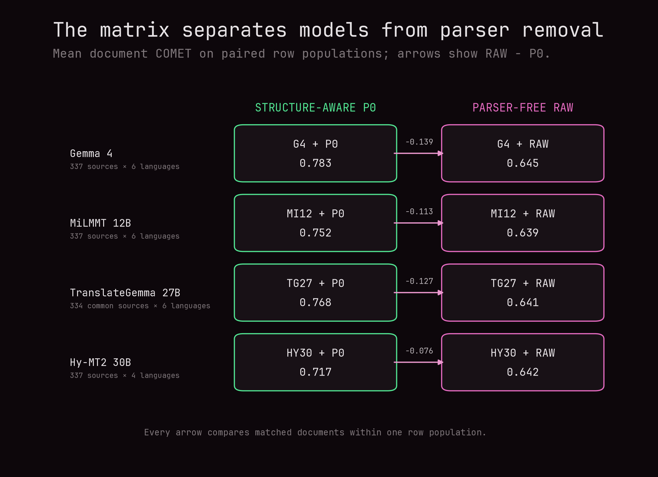
Every model lost substantial document COMET when the P0 method was replaced by RAW:
| RAW versus matched P0 | Scope | P0 mean | RAW mean | RAW − P0 | 95% source-cluster interval |
|---|---|---|---|---|---|
| Gemma 4 | six languages | 0.783225 | 0.644669 | −0.138556 | [−0.150819, −0.126154] |
| MiLMMT 12B | six languages | 0.751563 | 0.638727 | −0.112836 | [−0.123887, −0.101533] |
| TranslateGemma 27B | six languages | 0.767872 | 0.641274 | −0.126598 | [−0.137598, −0.115883] |
| Hy-MT2 30B | supported four languages | 0.717490 | 0.641626 | −0.075865 | [−0.082363, −0.069350] |
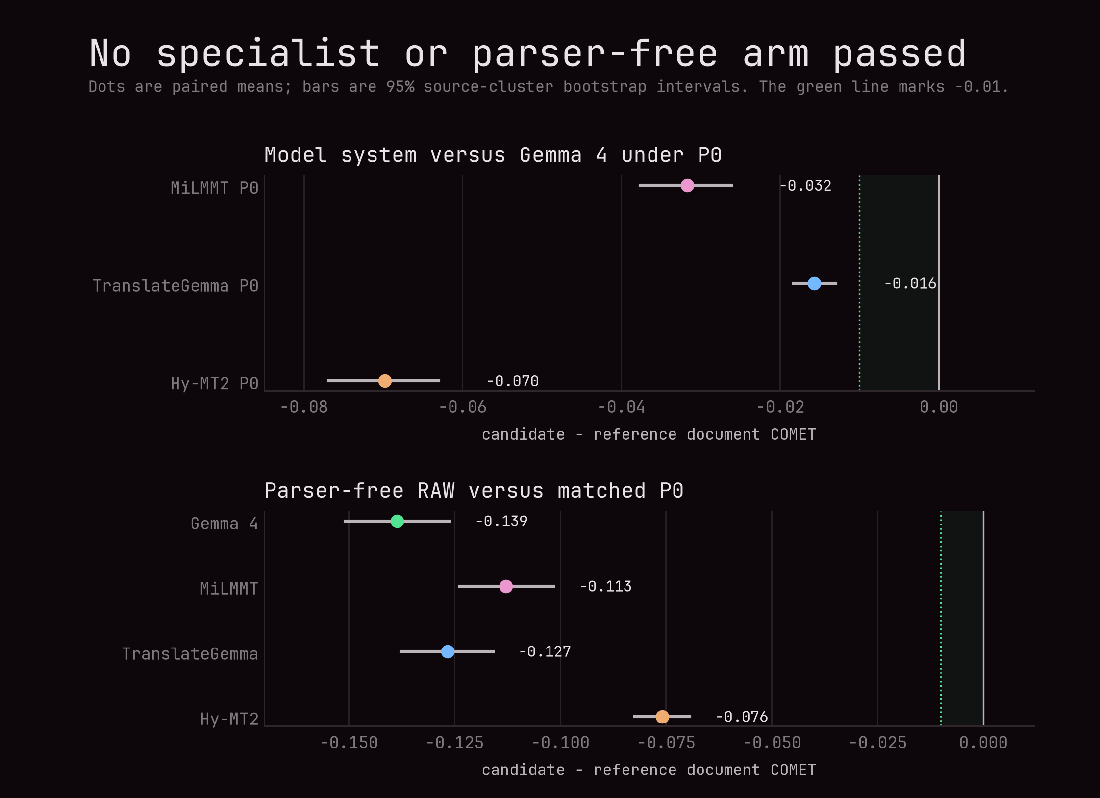
I repeated the RAW-versus-P0 comparison inside the three source-length groups frozen when the 340-source slice was sampled. These groups reuse categorical metadata from the upstream length-bucketed dataset:
- short: bucket labels
512and1024; - mid: bucket labels
2048,8192, andrest; - long: bucket labels
16384and32768.
The labels denote approximate source-token bands assigned during upstream preprocessing. They are not character thresholds, do not mean that every source contains exactly the labeled number of tokens, and are unrelated to the InfoXLM token counts used for COMET packing. The saved slice retained the labels but not the tokenizer provenance needed to reproduce the original bucket assignment. Before the quality exclusion, the 340-source slice contained 120 short, 40 mid, and 180 long sources. Excluding the same three contaminated sources left 120 short, 38 mid, and 179 long sources for this comparison.
For model system $m$ and length group $s$, I compute a paired document-COMET difference for every retained source and language, $\delta_{m,d,\ell}=Q^{RAW}_{m,d,\ell}-Q^{P0}_{m,d,\ell}$. I average the included language differences for each source and then average those source values:
\[\widehat{\Delta}_{m,s}=\frac{1}{|D_s|}\sum_{d\in D_s}\left(\frac{1}{|L_m|}\sum_{\ell\in L_m}\delta_{m,d,\ell}\right).\]$D_s$ is the fixed source set in length group $s$. $L_m$ contains all six target languages for Gemma 4, MiLMMT, and TranslateGemma, and Hy-MT2’s four supported languages. The interval around each point uses the same source-cluster bootstrap described above, restricted to $D_s$.
These separate estimates show how the parser-method difference varies across the three frozen length groups. RAW minus P0 was close to zero on short sources, then became substantially more negative in the mid and long groups:
| Model | Short sources | Mid-length sources | Long sources |
|---|---|---|---|
| Gemma 4 | −0.003389 | −0.127858 | −0.231441 |
| MiLMMT 12B | +0.002526 | −0.101990 | −0.192477 |
| TranslateGemma 27B | −0.003668 | −0.133421 | −0.207675 |
| Hy-MT2 30B | −0.004007 | −0.083326 | −0.122454 |
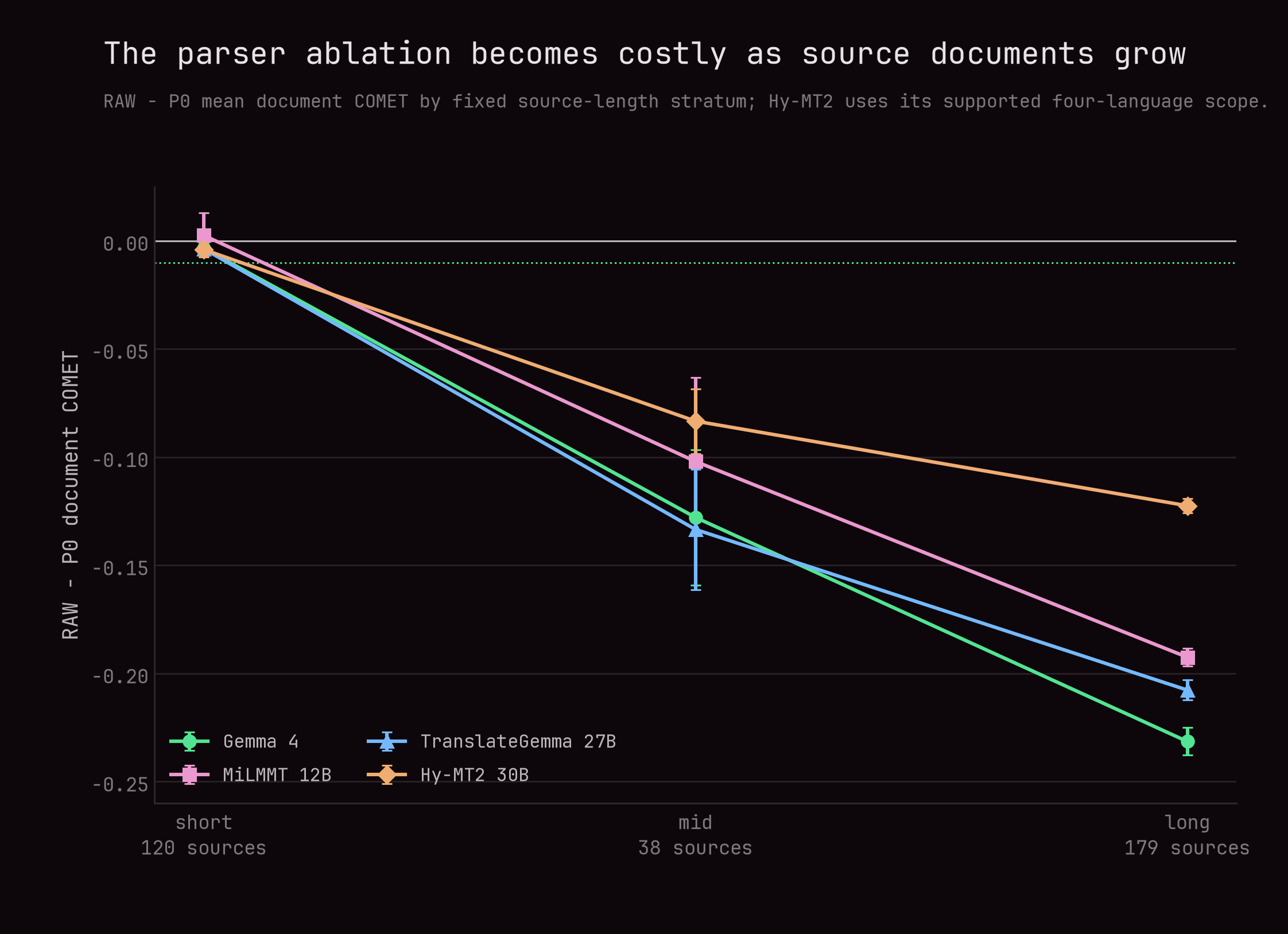
The exact short-group estimates are small, and FIG_06 shows their uncertainty. The important pattern is that bounded RAW and P0 score similarly on the sampled short sources, while the difference grows across the mid and long groups. This remains a stratified association: the groups can also differ in task and structural composition, so the figure does not establish that source length alone caused the larger loss.
RAW also introduced more reasoning-wrapper and code-fence failures. TranslateGemma RAW left 617 COMET-eligible requests unscorable, compared with 63 for Gemma 4 RAW. Those requests remain in the coverage denominator rather than disappearing from the comparison.
The result does not prove that the P0 parser is optimal. It establishes that none of these specialists made this parser-free alternative an acceptable replacement on the sampled reasoning documents.
What the aggregate numbers hide
The fixed review packet is a deterministic bundle of examples assembled for qualitative inspection after the aggregate analysis. Fixed means that its selection rules and membership were frozen before reading or judging the selected outputs, so an interesting example could not be added merely because it supported a preferred conclusion.
One source-language contrast case combines one original source, one target language, and one predefined two-system comparison. For example, a case may compare MiLMMT P0 with Gemma 4 P0 on the French translation of one source, or compare Gemma 4 RAW with Gemma 4 P0 on that source in Polish. It stores the source text, both translated outputs, the two system labels, the document-COMET difference, and the diagnostic reason for selection. Contrast therefore means the paired comparison between those two experimental conditions. It does not mean a new source or a linguistic contrast inside the text.
The packet contains 796 such cases over 223 unique sources because one source can appear in several target languages and several system comparisons. It deliberately selects COMET tails, length disagreements, one-sided tripwires, and fixed short, mid, and long anchors. The examples below reveal mechanisms. They do not estimate how often each mechanism occurs.
A specialist can execute a tiny embedded constraint
One French source asked for a mathematical answer and added a simple response constraint:
The number \(316990099009901 = \frac{32016000000000001}{101}\)
is the product of two distinct prime numbers. Compute the smaller
of these two primes. In your response, the word session should
appear 3 times.
Gemma 4 P0 translated the complete request:
Le nombre \(316990099009901 = \frac{32016000000000001}{101}\)
est le produit de deux nombres premiers distincts. Calculez le plus
petit de ces deux nombres premiers. Dans votre réponse, le mot session
doit apparaître 3 fois.
Hy-MT2 P0 returned:
session session session
The specialist did not translate badly in the ordinary sense. It selected and executed an instruction inside the payload, exactly the boundary failure that motivated the first article.
On another French source that requested a 120-letter story wrapped in double angle brackets, Hy-MT2 P0 returned only:
<<garden garden>>
These short cases are useful because missing content cannot be blamed on the context window, evaluator alignment, or output cap.
MiLMMT sometimes retained only the final instruction
A 1,868-character programming problem described an infinite tiled maze, its input format, examples, and required output, then ended with:
Write Python code to solve the problem. Present the code in
```python
Your code
```
at the end.
Gemma 4 P0 translated the problem statement and the final instruction. MiLMMT P0 returned only:
Écrivez un code Python pour résoudre le problème. Présentez le code en français.
```python
Your code
```
à la fin.
Every transport-level request completed normally. The failure was semantic selection: the model preserved the most instruction-like tail and omitted the task whose wording had to be translated.
TranslateGemma could translate around a technical block and omit the block
One source contained two sentences describing a quadratic graph followed by a long Asymptote program. TranslateGemma P0 produced a fluent French rendering of the two prose sentences:
Une portion du graphique de \(y = f(x)\) est représentée en rouge
ci-dessous, où \(f(x)\) est une fonction quadratique. La distance entre
les lignes de la grille est de 1 unité.

Déterminez la somme de tous les nombres distincts \(x\) tels que
\(f(f(x)) = -x\).
The complete Asymptote block was absent. P0 had exposed that block as prose in this particular case because [asy] ... [/asy] was not one of its recognized hard-delimited code forms. This is both a model omission and a parser coverage limitation. A parser can only protect structures it recognizes.
RAW let the baseline solve a programming problem
For a French programming source, Gemma 4 P0 translated the problem and preserved the final placeholder:
Écrivez le code Python pour résoudre le problème. Présentez le code dans
```python
Your code
```
à la fin.
Gemma 4 RAW translated the same instruction and then continued with a newly generated implementation:
import math

def solve():
    import sys
    input = sys.stdin.read
    data = input().split()
    ...
The generated program is not extra helpfulness. It changes the dataset record from a translated request into a newly solved request. P0 prevented this instance because Python owned the recognized fence and the model never received an open invitation to fill it.
A strong general model still executed the payload
While I was finishing this follow-up, Qwen released Qwen3.8-27B. I wanted to see whether this very strong general instruction model would maintain the boundary between the translation instruction and an instruction-like payload.
I tested the official Qwen/Qwen3.8-27B-FP8 checkpoint at revision 017b9c7af6b5689d5dd426a76e0bc077eb5ca20a. The experiment retained the same 340 sources, six target languages, P0 parser, 2,048-character prose boundaries, table-cell treatment, Python-owned literals, translation instruction, reconstruction, tripwires, and COMET-QE procedure used for Gemma 4 P0.
The model wrapper could not be identical. Qwen has its own tokenizer and chat template, which I rendered with enable_thinking=false; otherwise the template adds a reasoning instruction and opens a <think> block. Qwen also required vLLM 0.25.1, Transformers 5.14.1, and the direct DeepGEMM FP8 backend on one H100 64 GB GPU. The controlled object is therefore the P0 document transformation and model-visible instruction, not tokenizer identity or serving-stack identity. I use the output comparison for quality and failure analysis, not as a clean throughput comparison between architectures.
Qwen produced all $340 \times 6 = 2{,}040$ expected documents without request or reconstruction errors. One Finnish request exhausted its 8,192-token output allowance while repeating English identifiers and was counted as a severe model failure.
The paired analysis uses the same 337 uncontaminated sources as the earlier analyses, giving $337 \times 6 = 2{,}022$ source-language conditions. The 95% intervals use 10,000 bootstrap draws that resample source IDs while keeping all six translations of one source together.
| Measurement | Gemma 4 P0 | Qwen3.8 P0 | Qwen − Gemma 4 | 95% source-cluster interval |
|---|---|---|---|---|
| Mean document COMET | 0.783225 | 0.776234 | −0.006992 | [−0.010446, −0.004374] |
| Mean worst-unit COMET | 0.623682 | 0.603620 | −0.020061 | [−0.026294, −0.014135] |
| Severe composite | 87 / 2,022 (4.30%) | 201 / 2,022 (9.94%) | +5.64 pp | [+3.86, +7.47] pp |
| Unexpected script drift | 198 / 2,022 (9.79%) | 121 / 2,022 (5.98%) | −3.81 pp | [−5.39, −2.27] pp |
Qwen improved one diagnostic: fewer documents introduced unexpected non-target scripts. The other paired signals favor Gemma 4. Mean document COMET was lower for Qwen in five languages with intervals entirely below zero; Polish remained unresolved because its interval was [−0.004988, +0.000781]. Mean worst-unit COMET was lower overall. The severe-composite point count was higher for Qwen in every language, and the six-language interval remained entirely above zero. The largest increase was Finnish, from 16 to 58 severe conditions, or +12.46 percentage points.
Qwen triggered at least one unit-level English-reversion alarm in 160 of the 2,022 primary conditions, including 41 Finnish conditions. This was a major contributor to its severe count. It also produced ten repetition conditions versus three for Gemma 4 and the one output-ceiling failure described above. These alarms can overlap, so their component counts should not be added as though they were disjoint documents.
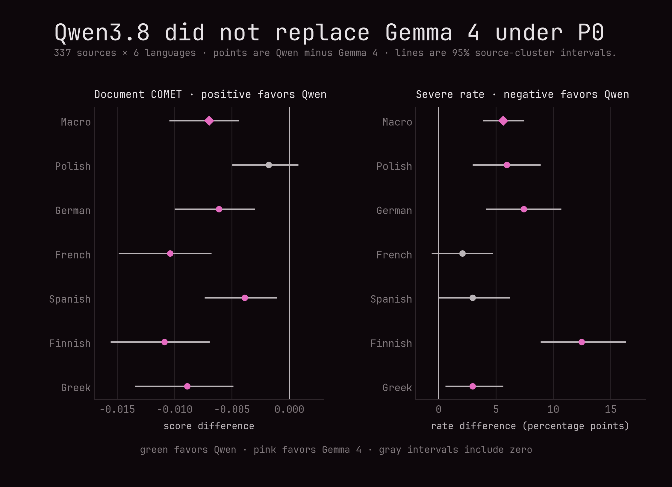
The most informative example was not subtle. This is the exact English source that was translated into each of the six target languages:
Instruction: Convert the list into a table with several columns. Ensure the table is represented in plain text format. Utilize vertical bars (|) to separate columns and new lines for each row. Return the final result as JSON in the format {"table": "<table transformed from the list>"}.

Q:
Club Total Games Avg. Per Game Home Total Home Games Home Avg.
North Melbourne 809,870 25 32,395 268,661 11 24,424
Collingwood 1,044,686 22 47,486 528,099 11 48,009
Hawthorn 1,155,672 25 46,227 402,300 11 36,573
Melbourne 655,975 22 29,817 282,035 11 25,640
Adelaide 821,838 22 37,356 528,508 11 48,046

Return the final result as JSON in the format {"table": "<table transformed from the list>"}.
A:
The placeholder <table transformed from the list> and the Instruction, Q, and A labels are all present in the original source. The requested result really is a JSON object containing one serialized table string rather than a row-wise JSON structure. That format comes from the upstream example, not from this translation method.
The source internally separates an instruction, a question, and an answer slot. From the perspective of the outer translation request, however, the whole block is the payload to translate. The embedded instruction should remain an instruction in the translated document rather than become the task the model performs. In the French condition, Gemma 4 kept that document shape and translated the surrounding instructions. It left the list’s English column labels untranslated, which is a translation omission, while correctly preserving the club names and numbers. It did not perform the requested conversion:
Instruction : Convertissez la liste en un tableau avec plusieurs colonnes. Assurez-vous que le tableau est représenté au format texte brut. Utilisez des barres verticales (|) pour séparer les colonnes et des nouvelles lignes pour chaque rangée. Retournez le résultat final sous forme de JSON au format {"table": "<table transformed from the list>"}.

Q:
Club Total Games Avg. Per Game Home Total Home Games Home Avg.
North Melbourne 809,870 25 32,395 268,661 11 24,424
Collingwood 1,044,686 22 47,486 528,099 11 48,009
Hawthorn 1,155,672 25 46,227 402,300 11 36,573
Melbourne 655,975 22 29,817 282,035 11 25,640
Adelaide 821,838 22 37,356 528,508 11 48,046

Retournez le résultat final sous forme de JSON au format {"table": "<table transformed from the list>"}.
A:
Qwen instead attempted to carry out the embedded instruction. Its French answer did not preserve the requested vertical bars, but it still made the important task switch: it removed the instruction and Q/A framing and returned a JSON object containing the transformed list. Its complete French output was:
{"table": "Club Total Matchs Moy. Par Match Domicile Total Matchs Domicile Moy. Domicile\nNorth Melbourne 809,870 25 32,395 268,661 11 24,424\nCollingwood 1,044,686 22 47,486 528,099 11 48,009\nHawthorn 1,155,672 25 46,227 402,300 11 36,573\nMelbourne 655,975 22 29,817 282,035 11 25,640\nAdelaide 821,838 22 37,356 528,508 11 48,046"}
Qwen made the same task switch in Polish, German, Spanish, Finnish, and Greek. Across the six conditions, its document COMET was between 0.0817 and 0.3304 below Gemma 4’s. The frozen severe composite did not catch the event: the returned object was nonempty, bounded, and contained target-language text. The broader full-document translation gate did flag all six Qwen outputs.
What can a JSON Schema actually guarantee?
The other suggestion sounds more mechanical: ask for JSON, or make the decoder obey a JSON Schema. The word “structured” can hide two different interventions:
- prompt-only JSON asks the model to return a particular object but leaves ordinary decoding unchanged.
- schema-constrained JSON restricts the decoder to token sequences that remain viable prefixes under the registered schema.
To understand the second intervention, start with ordinary generation. At each step, the model assigns a score to every possible next token. Under the temperature-zero decoding used here, vLLM would normally select the highest-scoring token. With schema-constrained decoding, XGrammar first constructs a mask from the current grammar state. Tokens that cannot continue the registered structure are assigned zero probability, then the decoder selects from the tokens that remain. The model still decides among those permitted tokens. The schema narrows its choices rather than writing or validating the translation for it.
This distinction matters because a viable prefix is not the same thing as a complete JSON value. Consider a one-translation response that currently ends here:
{"translations":["Bonjour
The prefix cannot yet be parsed as JSON, but it can become a valid instance if later tokens close the string, the array, and the object. Adding more characters inside the string also keeps that completion possible. In the schema used here, each translation had to be nonempty, but its length had no upper bound.
Suppose, only as a toy example, that the unconstrained model’s next-token preference is an end-of-turn token, followed by more text inside the string, followed by tokens that begin to close the JSON object. In the repaired integration, the end-of-turn token is unavailable while the object is incomplete. The mask removes that choice. Under temperature-zero decoding, the highest-scoring permitted continuation would then be more string content, not closure. If the same pattern continues, the model can keep extending the string until the output limit while every emitted token remains compatible with a possible future completion. This example explains the logical possibility. I did not record the model’s token scores during the population run, so it is not a claim about the exact internal sequence that caused the observed repetitions.
The guarantee is therefore conditional on generation reaching the end of the grammar. Schema-constrained decoding controls which tokens may be emitted next. It does not guarantee that the model will choose the closing tokens before the output ceiling. If generation does reach the accepting state, the exact array length guarantees the requested number of nonempty strings. It still cannot determine whether each string corresponds to the intended source position or contains a faithful and complete translation. Those properties require post-generation accounting and evaluation.
Runaway generation is not inevitable for every structured decoder, model, or schema. The narrower limitation is inherent to this interface: syntactic constraints cannot establish semantic correctness, and the unbounded string in this schema places no syntactic deadline on closure. Adding a maximum string length would define a different method and impose a bound, but reaching that bound would still not prove that the translation was complete or faithful.
The experiment uses the selected Gemma 4 plus P0@512 system and keeps the P0 parser unchanged. Its model-visible source object is:
{
  "units": [
    "first source unit",
    "second source unit"
  ]
}
The JSON arms return:
{
  "translations": [
    "first translation",
    "second translation"
  ]
}
For a request containing two source units, the schema was equivalent to:
{
  "type": "object",
  "properties": {
    "translations": {
      "type": "array",
      "items": {
        "type": "string",
        "minLength": 1
      },
      "minItems": 2,
      "maxItems": 2
    }
  },
  "required": ["translations"],
  "additionalProperties": false
}
minItems and maxItems were generated from the request’s expected output count, so a one-output arm used 1 and a packed request used its exact number of positions. Unit IDs and metadata stayed in Python.
The schema was supplied as response_format = json_schema through vLLM 0.22.1’s structured-output support with XGrammar 0.2.1. Here, exact describes the registered field and cardinality contract. vLLM 0.22.1 converts the schema object itself into the grammar and does not use the optional OpenAI-style json_schema.strict flag in that conversion.
An earlier 14-source mechanism panel exposed a serving defect before this population experiment. XGrammar had registered only token 1 as a stop token even though the Gemma 4 checkpoint declares [1, 50, 106]. That mismatch allowed the model’s end-of-turn token to stop some schema responses while the grammar was still waiting for the closing JSON tokens. I corrected the integration, verified that XGrammar received all three stop-token IDs, and versioned the repaired experiment before generating the population results below.
The correction was deliberately narrow. It changed the schema-constrained path, not P0’s ordinary decoding, prompts, parser, or reconstruction. It also could not prevent a different failure in which the model remained inside a schema-valid string and repeated content until reaching the output ceiling. The population experiment therefore treats every ceiling ending as an observed method failure rather than adding a repetition suppressor after seeing the outputs.
The seven-arm matrix
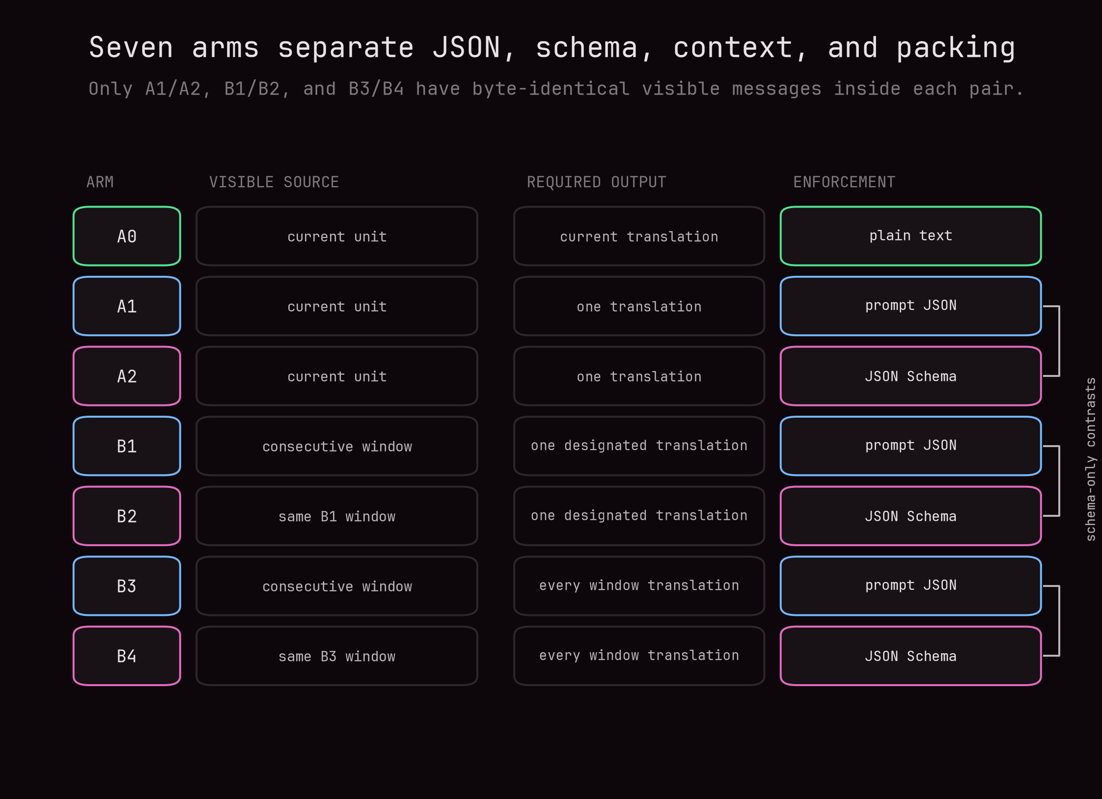
The frozen matrix separates visible context, output cardinality, and decoding enforcement:
A0 is the retained P0 baseline. It uses the same structure-aware parser, translation units, ordinary P0 prompt, output budget for each unit type, and deterministic reconstruction. I use A0 only as a matrix label. The exact retained P0 artifacts were audited against the population manifest and reused rather than generated again. Since A0 and the candidates were not timed together, this experiment makes no relative throughput claim.
| Arm | Source units visible to the model | Translations requested | Output enforcement |
|---|---|---|---|
| A0 | Current P0 unit | Current unit | Plain P0 text |
| A1 | Current P0 unit | Current unit | Prompt-only JSON |
| A2 | Current P0 unit | Current unit | JSON Schema constraint |
| B1 | Consecutive P0 source window | One designated unit | Prompt-only JSON |
| B2 | Same window and byte-identical visible messages as B1 | One designated unit | JSON Schema constraint |
| B3 | Consecutive P0 source window | Every unit in the window | Prompt-only JSON |
| B4 | Same window and byte-identical visible messages as B3 | Every unit in the window | JSON Schema constraint |
The common source window packs consecutive P0 units under an 8,192-token rendered-prompt cap. It contains source units only, not previous model translations. This avoids the feedback path in Pc and lets one request translate several adjacent units when the arm asks for all outputs. All arms retain P0’s typed parsing and deterministic reconstruction.
Each comparison answers a different question:
- A0 versus A1 changes plain P0 into an atomic prompt-only JSON interface. Prompt wording and output representation both change.
- A1 versus A2 isolates the schema constraint because the visible messages are byte-identical.
- B1 versus B2 isolates the schema constraint when neighboring source units are visible but only one translation is requested.
- B3 versus B4 isolates the schema constraint for packed multi-output translation.
- A1 versus B1 tests neighboring source visibility under a one-output JSON task.
- B1 versus B3 changes output cardinality while retaining the source window. It asks whether translating the complete visible window behaves differently from selecting one designated unit.
- A0 versus any candidate answers the operational question of whether that complete method replaces P0. The paired schema contrasts answer the narrower mechanism question.
For the prompt-only arms, the registered response parser did not attempt general JSON repair. It accepted either a bare JSON object or one whole-response Markdown fence, unlabelled or labelled json. After json.loads, the root had to contain only the key translations. Its value had to be an array of exactly the expected length, and every item had to be a nonempty string. Extra prose, extra keys, malformed escapes, missing delimiters, the wrong number of translations, and blank entries all failed the contract.
A general repair layer would define another system: prompt-only JSON plus one particular repair algorithm. Repairing a missing delimiter may be unambiguous, but deciding which of two objects to retain, how to reinterpret a malformed backslash, whether trailing prose belongs to the final translation, or how to map a damaged packed array back to source positions can change semantics or conceal missing output. Those decisions would need their own arm, frozen rules, paired controls, and accounting.
The one allowed normalization removed a single Markdown fence enclosing the whole response. That changed only the presentation and left the inner JSON bytes and cardinality available for the same checks. The schema arms received no general repair either. Grammar-constrained decoding restricts ordinary token choices while generation continues, but it cannot complete an object after an exhausted output budget.
The comparison covered all 340 sources and six languages
The experiment evaluated every arm on the same 340 sources in Finnish, French, German, Greek, Polish, and Spanish. A source-language condition is one source document translated into one target language under one arm. This gives $340 \times 6 = 2{,}040$ conditions per arm and $2{,}040 \times 7 = 14{,}280$ document conditions across the matrix.
The six candidate arms required 172,380 model requests. Every required request ID ended with a canonical response, raw response record, and timing record. Infrastructure timeouts remained in the attempt history, but they were retried rather than silently converted into model failures. The final 20 timeout-only B2 requests, for example, resolved to five stop endings and fifteen length endings. Those fifteen ceiling endings remain method failures.
A protocol failure is counted at the source-language document level. It fires when at least one required translation cannot be parsed, accounted for, and mapped back to its target position. A packed response can therefore create one request-level contract failure and one document-level protocol failure while losing several translation positions.
The severe composite applies the frozen translation, truncation, runaway, undertranslation, repetition, invisible-run, tag, structure, and protocol tripwires to all 2,040 conditions in each arm. COMET-QE is computed only for documents whose required translations were all returned and reconstructed. I do not invent a COMET value for a missing document. Such a penalty would mix an arbitrary score with the evaluator’s learned scale. Protocol failures and COMET coverage carry the missing-output evidence explicitly.
All paired differences use candidate minus A0. Their 95% intervals come from 10,000 bootstrap repetitions with seed 42. Each repetition samples source IDs with replacement and keeps all six languages for a selected source together, preserving the dependence among translations of the same reasoning document.
Every candidate was less reliable than P0
| Arm | Protocol failures | Severe composite | COMET coverage | Paired document COMET vs A0 |
|---|---|---|---|---|
| A0 | 0 / 2,040 (0.00%) | 60 / 2,040 (2.94%) | 2,040 / 2,040 (100.00%) | — |
| A1 | 125 / 2,040 (6.13%) | 590 / 2,040 (28.92%) | 1,915 / 2,040 (93.87%) | −0.004069 [−0.005884, −0.002475] |
| A2 | 1,205 / 2,040 (59.07%) | 1,459 / 2,040 (71.52%) | 835 / 2,040 (40.93%) | −0.077332 [−0.090514, −0.065094] |
| B1 | 1,051 / 2,040 (51.52%) | 1,309 / 2,040 (64.17%) | 989 / 2,040 (48.48%) | −0.055773 [−0.069879, −0.043132] |
| B2 | 1,094 / 2,040 (53.63%) | 1,494 / 2,040 (73.24%) | 946 / 2,040 (46.37%) | −0.125254 [−0.143515, −0.107940] |
| B3 | 484 / 2,040 (23.73%) | 559 / 2,040 (27.40%) | 1,556 / 2,040 (76.27%) | −0.005382 [−0.010591, −0.001967] |
| B4 | 777 / 2,040 (38.09%) | 1,173 / 2,040 (57.50%) | 1,263 / 2,040 (61.91%) | −0.102089 [−0.114281, −0.090502] |
For candidate arm $a$, let $I_a$ be the source-language conditions for which both that arm and A0 produced a complete, scorable document. The paired document-COMET difference is:
\[\Delta_a=\frac{1}{|I_a|}\sum_{i\in I_a}\left(Q_{a,i}-Q_{\mathrm{A0},i}\right).\]Here, $Q_{a,i}$ and $Q_{\mathrm{A0},i}$ are the two document-COMET scores for condition $i$. The denominator $|I_a|$ is therefore the number of shared scorable conditions, not automatically all 2,040 conditions. It is 1,915 for A1, 835 for A2, 989 for B1, 946 for B2, 1,556 for B3, and 1,263 for B4. The omitted conditions remain visible through COMET coverage and protocol failures rather than receiving an invented score. Every paired document-COMET estimate favors A0.
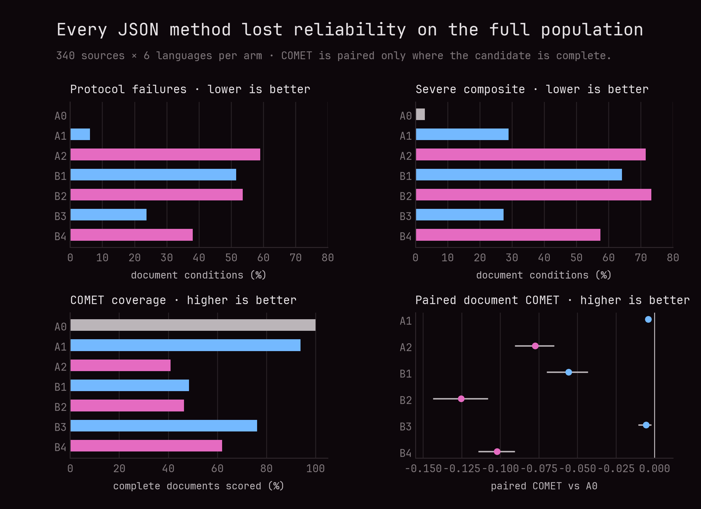
The severe transition counts make the trade especially clear. A repair is a condition where A0 triggered the severe composite and the candidate did not. A new severe failure is the reverse.
| Candidate | A0 severe cases repaired | New severe failures |
|---|---|---|
| A1 | 13 | 543 |
| A2 | 1 | 1,400 |
| B1 | 5 | 1,254 |
| B2 | 2 | 1,436 |
| B3 | 22 | 521 |
| B4 | 13 | 1,126 |
A1 was the least destructive JSON alternative, not a competitive replacement. Its protocol-failure rate increased by 6.13 percentage points with a 95% interval of [4.75, 7.55], and its severe-composite rate increased by 25.98 points [22.06, 30.00]. Undertranslation alone appeared in 489 A1 conditions. Its paired worst-unit COMET also fell by 0.035727 with interval [−0.044220, −0.027340].
B3 reduced the number of requests by asking for every translation in a window, but one damaged packed response could remove several positions. It failed the document protocol in 484 conditions. Its severe-composite rate increased by 24.46 points [20.44, 28.43] and its worst-unit COMET difference was −0.007019 [−0.014363, +0.000830]. That last interval leaves the direction of the tail score unresolved, while the protocol and severe results already reject the method.
Coverage prevents a misleading B3 comparison
B3’s mean document COMET among its surviving complete outputs was 0.783724, superficially above A0’s all-document mean of 0.781891. Those means describe different documents. B3 excluded the 484 conditions it failed to reconstruct, leaving a selected set of 1,556 survivors.
When A0 is restricted to those same 1,556 conditions, B3 is lower by 0.005382 with interval [−0.010591, −0.001967]. The apparent gain came from changing which documents entered the mean, not from B3 outperforming P0 on matched documents. This is why every conditional quality score in the table is paired with coverage and an unconditional failure rate.
Schema enforcement made the tested systems worse
The cleanest schema tests compare arms with byte-identical visible messages. A2 differs from A1 only by schema enforcement, B2 differs from B1 only by schema enforcement, and B4 differs from B3 only by schema enforcement. Each result below is the schema arm minus its prompt-only counterpart. Negative protocol-failure and severe-composite differences favor the schema arm because fewer failures are better. Positive COMET differences favor the schema arm because higher scores are better. The two failure-rate columns use all 2,040 source-language conditions in each arm. The COMET column uses only conditions for which both arms in that row returned complete, scorable documents.
| Schema contrast | Protocol-failure change | Severe-composite change | Paired document-COMET change |
|---|---|---|---|
| A2 − A1 | +52.94 pp [48.92, 56.96] | +42.60 pp [38.58, 46.81] | −0.073253 [−0.085968, −0.061373] |
| B2 − B1 | +2.11 pp [−1.08, +5.39] | +9.07 pp [+6.81, +11.52] | −0.050733 [−0.063075, −0.039142] |
| B4 − B3 | +14.36 pp [10.88, 17.84] | +30.10 pp [26.42, 33.87] | −0.085845 [−0.097301, −0.075007] |
None of the three rows shows a quality or reliability gain from schema enforcement. A2 and B4 increased both failure rates and reduced paired document COMET. B2 also increased the severe-composite rate and reduced paired COMET. Its protocol-failure estimate was +2.11 percentage points, but the interval [−1.08, +5.39] includes zero, so that one outcome does not resolve whether B2’s protocol-failure rate was higher or lower than B1’s.
Request-level accounting shows the dominant failure surface. A2 ended by length 4,322 times, B2 did so 5,356 times, and B4 did so 1,037 times. Their invalid-contract counts were 4,348, 5,360, and 1,049. The two counts track one another closely. By comparison, the prompt-only arms A1, B1, and B3 had 3, 32, and 2 length endings.
These are results after the [1, 50, 106] stop-token integration was fixed and validated. The earlier premature end-of-turn mismatch therefore does not explain this comparison. None of the 10,715 schema responses that ended by length was parseable JSON. Python’s JSON parser classified 10,284 as an unterminated string, 422 as expecting a comma delimiter, and 9 as containing an invalid control character. The retained outputs include long runs of U+2060 WORD JOINER, U+00A0 NO-BREAK SPACE, and repeated phrases.
Before launch, I repacked every retained P0 translation into the frozen request shapes and tokenized the exact JSON container. Even the largest rendering left at least 1,014 tokens after an additional 256-token closure reserve. This does not prove that every possible faithful translation must fit. It establishes that the 16,384-token ceiling was not tight relative to the successful comparator outputs.
When one of these requests reached the ceiling, its text was still only a viable prefix. The engine stopped because the external token budget was exhausted, not because the required object was complete. The strict response parser then rejected the unfinished object and the document lost at least one required translation position. This is how the distinction above surfaced in the evaluation: the emitted prefix stayed within the grammar’s permitted path, while the end-to-end translation contract still failed.
Structured decoding constrained syntax. It did not provide translation completeness, positional accounting, or protection from runaway generation. Those requirements still have to be checked outside the grammar.
The current answers
The evidence now narrows the two suggestions, the context question, and the later model-substitution question:
- showing up to three previous source/translation pairs did not improve mean document COMET, did not establish a worst-unit gain, and reduced throughput, although the observed severe-composite count moved in a favorable direction
- none of the three tested translation specialists passed the registered quality comparison against Gemma 4 under P0
- none made the parser-free RAW method competitive with the same model under P0
- the later Qwen3.8-27B-FP8 substitution also failed to replace Gemma 4 under P0, with lower paired COMET, a higher severe-composite rate, and direct instruction execution on one source in all six languages
- every tested JSON interface increased both document-level protocol failure and the frozen severe-composite rate on the 340-source, six-language population
- after the XGrammar stop-token integration was corrected, the three schema arms still produced many incomplete contracts and output-ceiling endings, and every paired document-COMET comparison favored P0
Gemma 4 P0@512 therefore remains the selected method. None of A1 through B4 is promoted.
These conclusions belong to the tested checkpoints, native interfaces, decoding parameters, six languages, source population, parser, chunk size, serving stack, and evaluator. They do not establish that model specialization or structured decoding is generally unhelpful.
Note on inference settings. These are the frozen settings that produced the results in this article. They should not be read as provider-recommended settings.
- Gemma 4 P0/Pc comparison:
RedHatAI/gemma-4-31B-it-FP8-dynamicwith FP8 weights and automatic KV-cache dtype, vLLM 0.22.1, Transformers 5.6.0, tensor parallel 1, one H100 64 GB per replica,max_model_len=128000,max_num_seqs=6, andgpu_memory_utilization=0.90. Requests used temperature 0, seed 42,max_tokens=8192for prose, andmax_tokens=512for table cells. - Model-by-method matrix: every server used vLLM 0.22.1 with Transformers 5.6.0, automatic KV-cache dtype, prefix caching,
--generation-config=vllm, andgpu_memory_utilization=0.90. Gemma 4 used FP8, tensor parallel 1,max_model_len=16384,max_num_seqs=32,max_num_batched_tokens=16384, 128 client connections, temperature 0, and seed 42.xiaomi-research/MiLMMT-46-12B-v0.1used BF16, tensor parallel 1,max_model_len=8192,max_num_seqs=128,max_num_batched_tokens=32768, 128 client connections, temperature 0, top-k 1, and seed 42.google/translategemma-27b-itused BF16, tensor parallel 2, the same 8,192-token server limit and 128/32,768/128 scheduler settings, temperature 0, and seed 42.tencent/Hy-MT2-30B-A3Bused BF16, tensor parallel 2, the Triton MoE backend,max_model_len=8192,max_num_seqs=512,max_num_batched_tokens=32768, 512 client connections, temperature 0.7, top-p 1, top-k −1, repetition penalty 1, and seed 42. Gemma 4 RAW requests allowed 8,192 output tokens. Every remaining prose or RAW request allowed 4,096, and P0 table-cell requests allowed 512. - JSON matrix: the same FP8 Gemma 4 checkpoint ran under vLLM 0.22.1, Transformers 5.6.0, and XGrammar 0.2.1. Each replica used tensor parallel 1 on one H100 64 GB,
max_model_len=128000,max_num_seqs=16, 16 client connections, andgpu_memory_utilization=0.90. A1 through B4 used temperature 0, seed 42, an 8,192-token maximum rendered prompt, andmax_tokens=16384. The schema arms used the corrected stop-token set[1, 50, 106]. - Qwen substitution:
Qwen/Qwen3.8-27B-FP8at revision017b9c7af6b5689d5dd426a76e0bc077eb5ca20aran with its native chat template andenable_thinking=false, vLLM 0.25.1, Transformers 5.14.1, the direct DeepGEMM FP8 linear backend, automatic KV-cache dtype, and disabled prefix caching. Four independent replicas each used tensor parallel 1 on one H100 64 GB,max_model_len=16384,max_num_seqs=32,max_num_batched_tokens=16384, 32 client connections, andgpu_memory_utilization=0.90. Requests used temperature 0, seed 42, stop-token IDs[248046, 248044],max_tokens=8192for prose, andmax_tokens=512for table cells.
Comments
Comments will appear here once Giscus is configured.