On this page
The project stopped being a throughput project when I opened one of the fast outputs and found an answer.
I was translating a large reasoning dataset into several European languages. The serving stack looked healthy. Requests completed. The inference server returned finish_reason = stop. Output files had the expected number of rows. The translated text had plausible length. Everything looked fine from the outside. Then I read the samples.
Inside some of the rows, the model had silently changed jobs. A source example asked for a proof, a program, or a mathematical derivation. The translation prompt asked the model to translate that example. The model sometimes followed the instruction embedded in the source and solved the problem instead. In other cases it restated the prompt, wrote a concise answer, or replaced a long reasoning trace with a much shorter piece of helpful prose.
This failure matters well beyond one dataset. Translation, rewriting, proofreading, and summarization all place an instruction following model in a peculiar position: the input contains language that must be treated as data, while the surrounding prompt asks for a transformation. Recent work calls the broader phenomenon instructional distraction. Reasoning corpora make the boundary especially fragile because the text being transformed often looks exactly like the kind of task the model was trained to execute.
What follows is the engineering and evaluation story of that failure. It starts with a throughput benchmark, passes through three generations of chunking and structure preservation, and ends with a bounded launch recommendation. The result is less satisfying than a universal recipe. It is also more useful: one small operating region survived every check I could run, while larger chunks failed sharply and context variants made the translations worse.
A small, cleaned-up implementation of the translation and evaluation workflow is available in ReinforcedKnowledge/translation-lab.
The object being translated
Dolci-Think-SFT-7B is a post-training dataset with more than two million examples. Its defining structure is a reasoning trace inside <think> tags followed by a final answer after the closing tag. A simplified row looks like this:
user:
Write a Python program that solves ...

assistant:
<think>
We need derive the algorithm. First observe ...
</think>
Here is the implementation:
```python
...
```
The translation contract sounds simple until its invariants are written down. The target should preserve the conversation schema. It should contain exactly one reasoning block when the source contains one. The final answer should remain outside that block. Natural language should move into the target language. Code, identifiers, display mathematics, and markup should survive without creative edits. Most importantly, the transformed row should retain the source intent. A request to write a program must remain a translated request to write a program. Turning it into a newly written program breaks the contract.
I use row for one dataset record: the user message, the assistant reasoning, the final answer, and the associated metadata. I use source document for the assistant content inside that row, since that is the material sent to the translation pipeline. In the experiments below, one row contributes one source document. A full-document method translates it in one request, while a chunked method divides the same document into several requests and reconstructs one output row.
I use hijack for that last failure. A hijacked translation is an output in which the model executes, answers, summarizes, or otherwise takes over the instruction contained in the source. The term is behavioral and makes no claim about mechanism or malicious input. It says that the boundary between instruction and payload failed.
This makes quality part of throughput. If a run produces 100 rows per second and 20 of them are answers rather than translations, its useful throughput is below 80 rows per second. The exact correction is harsher because corrupt rows require detection, diagnosis, and often a rerun. Accepted translated tokens per GPU-hour is the quantity the project actually needs.
Long reasoning traces add a second problem. Many exceed one fixed inference budget, which turns translation granularity into an explicit tradeoff. Full-document translation has a strong coherence prior. Chunking creates more boundaries and more reconstruction work. It also gives the transformation instruction a better chance of remaining locally dominant.
That trade is the center of this article.
A normal stop is weak evidence
The first diagnostic mistake was treating server completion as task completion.
An OpenAI-compatible server usually reports stop when the model emits a stop token or reaches another ordinary termination condition. It reports length when the configured generation budget ends first. These signals answer a transport question. Did generation terminate normally under the serving contract? Semantic completion needs a separate question. Did the model translate the entire source?
A hijacked output can be internally complete. Consider a 12,000-character reasoning trace whose first line asks for a proof. The model can return a polished 900-character proof, close every fence, and stop naturally. The response is well formed. Its latency is excellent. Its token count is low. Every naïve operational metric rewards it.
This is why the initial symptom looked like a throughput improvement. Shorter generations increased apparent samples per hour. The output-to-source character ratio exposed the contradiction. Let
\[ r_{len} = \frac{|y|}{|x|}, \]where \(x\) is the source text and \(y\) is the model output. Character length is crude across languages, and a ratio near one proves very little. A very low ratio is still a useful alarm: the model probably omitted most of the document, compressed it radically, or changed tasks. The ratio cannot distinguish among those explanations. It only tells me which outputs deserve inspection.
I assembled a 30-row diagnostic fixture from the severe failures in the first long-document run. The initial screen kept source documents longer than 5,000 characters whose output-to-source character ratio was below 0.3. The 0.3 cutoff was a pragmatic screening choice, not a calibrated boundary between correct and incorrect translation. It marked outputs shorter than 30 percent of their sources as severe enough to inspect while retaining a varied candidate pool. The rule produced 70 candidates from 96 long rows. A stricter cutoff would have defined a narrower set of extreme failures and answered a different diagnostic question.
I then selected 30 candidates in round-robin order across source collection and a rough content label. The source collection came from the record identifier. The content label was heuristic: code if the source contained fenced code or Python-like tokens, otherwise math if it contained common LaTeX markers, otherwise table if it contained many pipe characters, and otherwise general reasoning. The final fixture contained 15 code-labeled rows, 10 math-labeled rows, 1 table-labeled row, and 4 reasoning-labeled rows. These labels were used only to avoid selecting thirty similar failures. Real documents often contain several of these forms at once. I called the fixture broken30.
The name is important because the fixture was failure-selected and designed for diagnosis. A separate reading of older production outputs estimated that roughly 6 to 9 percent of long reasoning rows showed severe whole-document hijack, while more than 90 percent translated faithfully. The percentage refers to the fraction of long rows in the failure class. It is not an output-to-source ratio, and it is not an estimate derived from broken30. The fixture answered a narrower question: can a candidate method recover examples we already know are difficult?
That distinction prevents one of the easiest evaluation errors in systems work. A stress fixture is useful for intervention development. It cannot be reported as an unbiased test set.
V1 as an intervention study
The first chunking experiment kept the pipeline simple. It compared five arms over the same 30 rows. Protection meant replacing fenced code, display and inline mathematics, boxed expressions, inline code, and table-like blocks with markers before translation, then restoring the saved spans afterward. Independent chunks meant splitting a document near paragraph boundaries into pieces of about 1,200 characters and translating each piece with no earlier document text. Previous context meant translating those chunks sequentially and showing the previous two source and translation pairs as read-only context for terminology and continuity. The model was asked to generate only the current chunk. The final arm combined context with protected spans.
| Arm | Input treatment | Passed the coarse translation gate | Mean output/source ratio |
|---|---|---|---|
| M0 | Full document, no protection | 2 of 30 | 0.22 |
| Mfp | Full document, protected spans | 4 of 30 | 0.30 |
| Mc0 | Small chunks, independent | 30 of 30 | 1.06 |
| Mcc | Small chunks, previous context | 30 of 30 | 1.06 |
| Mccp | Small chunks, previous context, protected spans | 30 of 30 | 1.07 |
The coarse gate, called looks_translated, tested three things at this stage: a plausible output-to-source length ratio, enough common target-language words in the prose, and no newly emitted code fence. A new code fence means that the output introduced a triple-backtick block where the source had none, a common signature when the model answered a programming request. Later versions added explicit checks for English reversion and script drift. English reversion means that translated prose stays in English or returns to English after beginning in the target language. The check compares common English and target-language word evidence after code and mathematics are removed. Script drift means that the output adds substantial text in an unexpected writing system, such as Cyrillic or CJK characters in a Polish translation, relative to what was already present in the source. These are high-recall alarms with known blind spots, not definitions of translation quality.
At this stage the result was still unmistakable on the selected fixture. Full-document prompting reproduced the gross failure. Small chunks cleared the tripwire on every row.
The useful causal claim is limited to that intervention. Smaller local payloads strongly reduced hijack on a failure-selected set. Context, placeholder protection, prompt wording, and reconstruction changed together in several arms, so their independent effects remain unresolved. Mc0, Mcc, and Mccp each passed 30 of 30 rows and had nearly identical mean length ratios. Those are the only similar measurements shown in the table. They do not tell us whether one method preserved meaning more accurately, omitted fewer details, used more consistent terminology, or produced better cross-chunk prose. I use fidelity for that semantic preservation and completeness.
An early analysis appeared to show that placeholder protection was harmful. The protection code replaced saved spans with markers such as ⟦CODE_0⟧, and the prompt instructed the model to reproduce the markers exactly. The same prompt also contained the generic example ⟦PH_n⟧. Models sometimes copied that example or changed a real marker toward its shape. Wrapper and stitching errors created additional marker-like artifacts. A counter that reported missing or malformed placeholders therefore mixed several causes: model corruption of a real marker, copying from the prompt, and mistakes in our own reconstruction code.
The resulting count answered only one question: did every marker created for this document survive the entire pipeline unchanged? It could not identify where a mismatch came from. The model might have altered a real marker. It might have copied the generic marker from the prompt. The reconstruction code might have lost or duplicated one while joining chunks. All three appeared as placeholder failures even though they imply different repairs.
To attribute a mismatch to placeholder protection itself, the prompt must contain no placeholder-shaped examples, the detector must compare the output only with the exact markers created for the current document, and the protection and restoration code must round-trip those markers without involving a model. Synthetic outputs should then test deletion, alteration, duplication, and prompt copying as separate cases. V1 did not isolate those causes, so its placeholder counts showed that the end-to-end pipeline produced marker mismatches. They did not show that protecting code, mathematics, or tables was inherently harmful. I withdrew that conclusion.
Chunking had passed one narrow test. The evidence justified another experiment, not deployment. broken30 had been selected because full-document translation failed on it, so it could not estimate behavior on ordinary rows. The coarse gate also ignored tag placement, paragraph boundaries, exact code preservation, semantic fidelity, and cross-chunk consistency. The next pass examined reconstruction directly, and the later representative sample addressed the selection bias.
V2 and the reconstruction seam
The second method made the document grammar explicit. It split each assistant message into three logical regions:
- prose before the reasoning block,
- prose inside the reasoning block,
- prose after the reasoning block.
The model never saw the literal <think> wrappers. Python removed them before inference and reinserted exactly one opening and closing tag during reconstruction. Each region was divided into chunks near 1,200 source characters. The S0 variant translated every chunk independently. The Sc variant supplied the previous two source and target chunks as context, with each contextual snippet capped at 600 characters.
Owning the wrapper in deterministic code eliminated one class of format drift. It also made a more ordinary bug visible. The stitcher joined translated paragraphs with an empty string. Paragraph boundaries disappeared, producing 336 run-together seams across the 30 examples. Every row still passed the cheap translation gate.
That bug is a compact demonstration of why aggregate pass rates are dangerous. Language checks saw target-language prose. Length checks saw enough output. Tag checks saw exactly one reasoning block. None of them represented paragraph topology. The correct repair was almost embarrassingly small: preserve the original blank separator and join paragraphs with \n\n where that separator existed.
V2 still sent fenced code to the model. Comments could be translated, identifiers could move, and delimiters could be changed. A long-form reasoning dataset contains enough executable text that this was more than cosmetic. Translation quality required a parser that could distinguish content the model should transform from content the host program should own.
V3 and host-owned structure
The third method became the stable experimental baseline. It parses a document losslessly into prose, fenced code, display mathematics, and tables. Hard-delimited code and display math bypass the translation model. Table grids remain literal while textual cells can be translated. Inline code and inline math remain a residual risk because their boundaries are more ambiguous.
The parser also owns the reasoning wrapper. The model receives prose chunks without <think> tags. Reconstruction restores the original block position and validates the count. This turns several probabilistic obligations into deterministic ones.
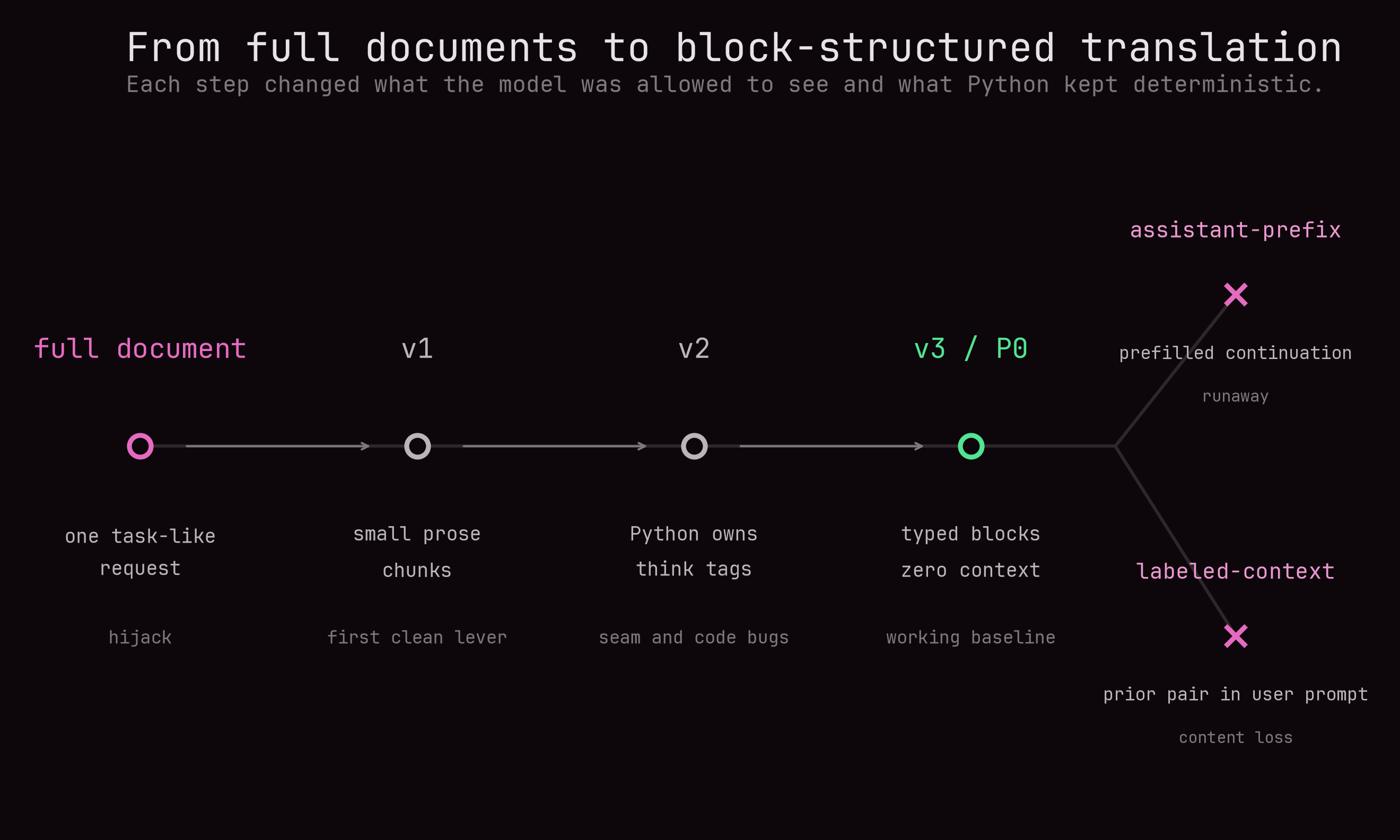
I call the independent variant P0. Each prose chunk is translated in isolation. I call the contextual variant Pc. Pc adds the previous three translated prose pairs as ordinary chat history. These names describe prompt topology only. They do not encode a model, language, or chunk size.
V3 also records the source and target text for every model call before reconstruction. These are known-by-construction pairs. That design decision later became essential for the exact quality-estimation model used here, wmt22-cometkiwi-da. Once separately translated pieces have been flattened into a document, recovering the exact correspondence is difficult. Evaluation is far more reliable when the pipeline preserves each source and translation pair at the moment it is created.
Chunk labels and real budgets
The experiment names chunk conditions with token-like labels: 300, 512, 1024, 2048, 4096, and 8192. The implementation actually splits on approximate source characters. The mapping is:
| Historical label | Approximate source characters | Maximum output tokens |
|---|---|---|
| 300 | 1,200 | 8,192 |
| 512 | 2,048 | 8,192 |
| 1,024 | 4,096 | 8,192 |
| 2,048 | 8,192 | 12,288 |
| 4,096 | 16,384 | 20,480 |
| 8,192 | 32,768 | 32,768 |
The labels are historical shorthand based on a rough conversion of four English characters per token. The splitter itself works in characters because it began as a simple, lossless text operation. It groups paragraphs, falls back to sentence or whitespace boundaries for oversized runs, and preserves the original separators for reconstruction. Tokenization was not avoided because it was computationally expensive. Its cost is negligible beside inference.
The inference engine tokenizes every prompt regardless of how the text was split. That step converts an already selected text chunk into model-specific token IDs. It does not choose the chunk’s textual boundary. If I had used each model’s tokenizer to enforce an exact token count, Gemma 3 and Gemma 4 would usually have received slightly different text spans under the same nominal condition. That would mix a model change with a segmentation change. This confound is avoidable: I could instead define boundaries once with a reference tokenizer, freeze those source spans, and then measure their realized lengths under every model tokenizer. The present study froze the existing character-based segmentation because the first curve had already used it. Changing the segmentation rule for only the later model would have prevented a direct comparison with that curve.
Character limits still require a token-level safety check. Before launch, a separate audit applies the exact chat template, tokenizes each completed prompt with the model’s own tokenizer, and verifies that the prompt plus its output allowance fits within max_model_len. Code, equations, punctuation, whitespace, and tokenizer choice all move the realized count away from the four-to-one estimate. If I were naming the experiment again, I would use the actual character budgets or rerun the entire curve with a tokenizer-aware splitter. I retain the token-like labels here only because they identify the recorded conditions.
The output budgets grow with the larger conditions. A length stop at label 4096 or 8192 cannot be explained by an accidentally tiny generation allowance. In practice, many of those cases are runaway continuations, task execution, or another form of loss of control. Large output budgets make that diagnosis clearer while increasing the cost of each failure.
A metric stack with narrow contracts
No single automatic metric identifies a correct translation of a mixed prose, code, mathematics, and reasoning document. I ended up treating evaluation as a stack. Every layer has a narrow contract and an explicit blind spot.
| Instrument | What it can catch | What it cannot establish |
|---|---|---|
| Structural checks | Missing reasoning tags, unbalanced fences, answer moved inside reasoning, wrapper leakage | Semantic fidelity |
looks_translated | Severe shortening, weak target-language evidence, English reversion, new fences | Fluent and complete translation |
nonlatin_drift | Newly introduced foreign-script runs relative to the source | Language identity for Latin-script languages |
| Language ID | Dominant document language after stripping code and math | Local untranslated spans and short-text quality |
| COMET-QE | Learned source and translation compatibility | A proof of correctness or completeness |
| Rubric review | Omissions, task execution, awkwardness, format damage | Native-speaker authority |
Structural checks
Structure is the easiest layer to make exact. The evaluation code counts reasoning tags, checks fence balance, verifies that the final answer remains outside reasoning, and looks for internal wrapper tokens in the model output. These tests are necessary because a structurally invalid row cannot be shipped. A perfectly structured answer to the wrong task still passes them.
looks_translated
The tripwire first strips code, mathematics, markup, and internal placeholders, then converts the remaining prose to lowercase word tokens. It combines several weak tests because no one of them identifies a translation.
The length test uses the number of output characters divided by the number of source characters. Its accepted interval, 0.6 to 1.6, was not derived from linguistic theory or fitted on a held-out calibration set. It began as a deliberately broad engineering band around a same-order-of-magnitude translation, then survived a retrospective audit of the saved outputs: most rows it rejected were genuinely truncated, gutted, or grossly expanded. It is still specific to this English-to-European-language workload. A legitimate expansion of a terse or symbolic source can exceed 1.6, and a full-length wrong answer can remain inside the band. The interval is an alarm threshold, not a universal property of translation.
The next test looks for common words from the requested language. In the notation below, tgt abbreviates target language. htgt is the number of remaining word tokens found in a small, manually curated list for that language, and nprose is the total number of remaining word tokens:
I require at least 25 prose word tokens before using this density as a pass or fail condition. Twenty-five is a pragmatic variance guard, not the result of an optimization sweep over 20, 25, and 30. It was introduced after inspection showed that the detector was falsely rejecting short, math-heavy translations. With a density bound of 0.10, a 25-token row needs at least three matching words to pass, whereas a 20-token row can pass on two. That does not make 25 universally correct. It makes the smallest accepted count less dependent on one or two word-list matches. Applying the guard, alongside better removal of code and mathematics and a corrected word list, reduced the short-stratum false alarm from 14 percent to 2 percent. For shorter prose, the gate records the density but does not reject the row merely because target-language evidence is weak.
For rows with at least 25 prose tokens, the gate needs a lower bound for what counts as enough target-language evidence. I calibrated that bound on code-stripped outputs. The lowest observed density among known-good translations was 0.172 for Polish, 0.195 for French, 0.178 for German, and 0.265 for Spanish. Hijacked Polish outputs had a median of 0.057, with many at zero. I placed the lower bound at 0.10, inside the observed gap. A density below 0.10 therefore raises a cheap gross-failure alarm. It does not measure fluency, adequacy, or completeness, and changing the word lists requires recalibrating the bound.
This is a target-presence test, not a general language detector. It asks whether the output contains enough evidence for the requested language. It does not identify which competing language dominates, and a failed test is an alarm rather than proof that the output is wrong. Finnish illustrates the limitation. Finnish often expresses grammatical relations with suffixes attached to content words, where languages such as French or English use separate articles and prepositions. For example, the ending in talossa expresses “in the house” without a separate word for “in.” An exact-match list of standalone function words therefore sees less evidence in perfectly valid Finnish prose. Faithful Finnish outputs can fall below 0.10, so Finnish relies more heavily on document-level language identification, COMET-QE, and review.
English reversion is checked separately because target-language and English evidence are not mutually exclusive. An output can translate its opening and conclusion, accumulate enough target-language matches to clear 0.10, and still leave a long reasoning passage in English. The detector therefore computes English density over the same stripped prose.
Two branches use different English-density bounds. When target-language evidence is absent, the detector raises an English-reversion alarm at 0.10. This reused the existing density bound as a symmetric minimum for clear English evidence. It was not independently optimized for English. That rule missed bilingual and partial-reversion outputs because they could contain enough words from both lists. I therefore added a second rule: English density of at least 0.15 raises the alarm even when target-language evidence is present. At the time of that change, faithful Polish and German outputs reached approximately 0.08 at most, while confirmed reverts began above 0.18. The value 0.15 was placed in that empirical gap. A later six-language audit found a faithful 99th percentile no higher than approximately 0.06 and zero false alarms at 0.15. Thus 0.06 is a reported property of the audit sample, 0.10 is the legacy English-only bound, and 0.15 is the partial-reversion bound. Common words shared by English and the target language are excluded from the English count where possible.
looks_translated is true only when the character ratio is inside the broad band, target-language evidence is not explicitly absent, English reversion is not detected, and the output has not introduced a code fence that the source lacked. New fenced code is an alarm because task execution often manifests as a fresh implementation. Fenceless code and very short task-execution responses remain blind spots.
The name looks_translated is intentionally modest. It is a runtime tripwire. Quality certification happens elsewhere.
Script drift and language ID
Here, script means a writing system represented by a Unicode character range, not executable code. The detector tracks Hangul syllables, Japanese kana, CJK ideographs, Cyrillic, and Greek. A script count is simply the number of characters in a text that fall inside one of those ranges. The set examined depends on the requested language. For Polish, French, German, Spanish, and Finnish, all five ranges are treated as foreign to the target’s Latin script. For Greek, Greek characters are expected, so the detector examines Hangul, kana, CJK, and Cyrillic instead. Latin is not treated as foreign to Greek because code identifiers, units, and names commonly use it.
For every writing system \(s\) tracked for that target, the detector compares its character count in the source, \(C_x(s)\), with the count in the output, \(C_y(s)\), and retains only a positive increase:
\[ D_s = \max(0, C_y(s) - C_x(s)). \]The stored nonlatin_drift value is the sum of those positive increases across the tracked ranges. The historical field name is slightly misleading because Greek characters are also tracked for Latin-language targets. Counting each writing system separately prevents a decrease in one source script from cancelling an increase in another. Unexpected CJK or Cyrillic runs in a French translation therefore become visible without penalizing the same characters when they were already present in the source. This remains a coarse proxy. Greek mathematical symbols can trigger false alarms, and drift between two Latin-script languages is invisible.
Post hoc language identification uses the pretrained model bundled with langid 1.1.6, the implementation described by Lui and Baldwin. It is a Naive Bayes classifier over byte n-gram features and returns the most likely ISO 639-1 language code from 97 supported languages. I run it on the reconstructed document after removing recognized code, mathematics, markup, and placeholders, then compare its predicted code with the requested target language. This is an analysis-only signal, not part of the runtime acceptance gate.
The classifier abstains when fewer than 30 Unicode letters remain. Thirty was not selected by a 20-versus-30-versus-40 accuracy sweep. It was added after tests showed that very short Finnish prose could be confused with Estonian and that emoji or residual mathematics could receive confident but meaningless predictions. Counting letters rather than all characters prevents digits, punctuation, and emoji from satisfying the floor. The value is a conservative hygiene rule for degenerate inputs, not a claim that every 30-letter passage is identifiable. Document-level outputs are normally far longer, so the rule mostly changes tiny or nearly prose-free cases. A production system that classified individual short chunks would need a dedicated length-calibration curve.
The classifier estimates the dominant document language, which is too blunt to find every local reversion. A long Polish document with one untranslated English paragraph will usually still be classified as Polish. That is why the document-level prediction supplements rather than replaces the English-density and script checks.
Three of the 340 sampled source rows contained enough CJK or code-switched natural language to confound these aggregate quality measures. I retained all three in the dataset and carved them out of language-quality aggregates, leaving 337 rows for the main estimates. The carve-out is part of the experiment manifest.
COMET-QE under a 504-token ceiling
COMET-QE adds a learned quality signal without requiring a human reference translation. The names around it are easy to collapse into one another, but they refer to different levels of the stack.
COMET is the general framework and model family for learned machine-translation evaluation. A reference-based COMET model can receive source, candidate translation, and human reference.
COMET-QE means reference-free quality estimation. At scoring time it compares the source with the candidate translation, without a human reference.
CometKiwi is a particular quality-estimation system built on COMET. It connects COMET with the predictor-estimator architecture from OpenKiwi and uses sentence-level and word-level QE objectives.
wmt22-cometkiwi-da is the released checkpoint used here. wmt22 identifies the WMT 2022 system and da identifies Direct Assessment, the human quality-score target behind its calibration.
The evaluator is wmt22-cometkiwi-da from the COMET project. The CometKiwi system paper describes the WMT quality-estimation system and its sentence-level and word-level objectives. Its encoder is based on InfoXLM.
The score is often discussed as if it lived cleanly between zero and one. The regressor can produce values outside that interval. More importantly, a scalar score inherits the evaluator’s tokenization and the evaluation pipeline’s alignment choices.
The tokenization in that sentence is COMET’s own, not a second tokenizer chosen for convenience and not the tokenizer used by the translation model. The scoring pipeline loads the InfoXLM tokenizer from the checkpoint and uses it both to count input tokens and to run the evaluator. Its subword boundaries determine whether a source and candidate pair fits, where an overlength pair must be divided, and the token weights used when unit scores are aggregated. A character counter or the translation model’s tokenizer would create different boundaries and could still send an overlength sequence to COMET.
At the Python interface, the expected input is a list of source and candidate-translation records:
[
    {
        "src": "English source span",
        "mt": "candidate translation span",
    }
]
Inside this checkpoint, the two fields are packed into one encoder sequence, with the candidate first:
<s> candidate translation </s></s> English source </s>
The encoder accepts 512 positions. The four special tokens in that template leave a hard maximum of 508 content tokens across both fields. The local evaluator uses 504, retaining a four-token safety margin. An unguarded overlength call is silently sliced to the encoder limit. Because the candidate appears first, this usually removes the tail of the source, precisely where a long translation may have diverged.
The checkpoint’s documented task is sentence-level quality estimation for natural-language machine translation. That evidence does not establish meaningful scoring behavior for serialized code, display mathematics, Markdown table grids, or control tags. I therefore do not claim that every such token was absent from every pretraining example. The narrower claim is that treating a score on those structures as evidence of translation quality would be unsupported. Identical code or mathematics can also dominate token overlap and inflate the document aggregate, while unfamiliar serialized structures can perturb it in the other direction.
The evaluator therefore removes fenced code, display math, tables, and bare control tags from both sides while retaining the reasoning prose. COMET-QE then measures natural-language source-to-translation compatibility. Separate exact checks remain responsible for code, mathematics, tables, tags, and reconstruction, so stripping those spans does not make them exempt from evaluation.
There are two stages after stripping: establish a source-to-translation correspondence, then pack each pair under the 504-token budget. For chunked translation, the source and translated chunk are saved together when they are produced, so the correspondence is known. For full-document translation, the evaluator extracts the source and output prose. It pairs corresponding prose blocks when both sides have the same number of blocks. If their block counts differ, it concatenates the prose on each side into one document-level pair before packing.
wholeexact pairA known pair already fits within 504 combined COMET tokens. Score it once without inventing a new boundary.
sentencealigned packingAn overlength pair has matching sentence counts. Pair sentence one with sentence one, then greedily merge adjacent pairs while they fit.
positionalapproximate fallbackWhen sentence pairing fails, split each side independently into pieces of at most 252 tokens and pair by order. The budget is exact; the semantic correspondence is approximate.
full-document prosepair constructionPair corresponding prose blocks when their counts match. Otherwise concatenate the source prose and output prose separately to form one document-level pair. Then apply one of the three packing modes above.
Here, whole labels an individual evaluation pair that fits. The original document may still have used many translation requests. The alignment label is stored with every evaluation unit, so approximate positional pairs can be separated from known or sentence-aligned pairs during analysis.
For a document with evaluation units $u$, I aggregate with token-length weights:
\[ Q_{doc} = \frac{\sum_u w_u Q_u}{\sum_u w_u}, \qquad w_u = T(src_u) + T(mt_u). \]Here, $Q_u$ is the COMET-QE score for evaluation unit $u$, and $w_u$ is that unit’s weight in the document average. $T(\cdot)$ counts content tokens with the same InfoXLM tokenizer used by the checkpoint, without adding the four fixed special tokens. Thus $T(src_u)$ is the token count of the source span in unit $u$, and $T(mt_u)$ is the token count of its candidate translation.
We do length weighting because evaluation-unit boundaries are partly an implementation detail. In an equal-unit average, every unit has one vote regardless of its size. Suppose two 400-token regions score 0.8 and 0.6. If each remains one unit, their unweighted average is 0.7. If the packer divides only the first region into four 100-token units, the average becomes $(0.8 + 0.8 + 0.8 + 0.8 + 0.6) / 5 = 0.76$. Nothing about the underlying document improved. The score changed because one region acquired four votes while the other retained one. This is the arbitrary-vote problem.
With token-length weights, the four 100-token units together retain approximately the same total influence as the original 400-token unit. Using source-plus-candidate length also reflects the amount of content placed in COMET’s joint encoder input. The obvious alternative is an equal-unit average, but that makes the result depend more strongly on how many pieces the packer happened to create.
There are two important limits. First, COMET is nonlinear. Scoring one 400-token pair is not generally equivalent to scoring four 100-token pairs and averaging them, even with exact length weights. Each call gives the encoder different surrounding context and can therefore produce different unit scores. Length weighting reduces the effect of the number of units, but it cannot make different segmentations mathematically equivalent.
Second, length weighting does not account for alignment confidence. A unit’s influence on the document score is $w_u / \sum_v w_v$. A positional pair containing 500 combined source and candidate tokens therefore has ten times the influence of a 50-token pair. This is intentional when both scores are equally trustworthy: the longer pair represents roughly ten times as much evaluated content.
The difficulty appears when the longer score is also less reliable. Write its observed score as
\[ Q_u = q_u + \varepsilon_u, \]where $q_u$ is the quality we want to measure and $\varepsilon_u$ is error introduced by imperfect correspondence between the source and candidate spans. In the document average, both terms are multiplied by the same factor, $w_u / \sum_v w_v$. Length weighting therefore scales both the useful quality signal and the alignment error. It has no confidence term telling it that one pair was matched exactly while another was assembled by an approximate positional fallback. Its implicit assumption is that a unit’s COMET-QE score represents all the content tokens in that unit and is about as trustworthy as scores from other units.
That assumption is weaker for positional pairs. Their source and candidate pieces are created independently and paired only by order. Expansion, omission, or a shifted boundary can make a large pair less semantically well matched even while its greater length gives the resulting score more influence. This risk grows in the large-chunk conditions because more material exceeds the evaluator’s budget and falls back to positional packing.
Combined-token-length weighting therefore solves the arbitrary-vote problem, not the alignment problem. Equal-unit averaging would cap each questionable pair at one vote, but it would reintroduce sensitivity to segmentation count: dividing the same passage into more pieces would give it more influence. A confidence-adjusted weight such as $w_u c_u$ could in principle combine content length with an alignment-confidence estimate $c_u$, but that estimate would itself require calibration against trustworthy alignments. I do not have that calibration here. I retain length weighting, interpret it alongside the alignment-method distribution and min_unit, and treat large-chunk COMET as comparative evidence rather than an absolute quality measurement.
I also store min_unit, the lowest unit score in the document. The mean can hide one collapsed tail segment. min_unit is a tail alarm.
A synthetic backstop tested four behaviors. Correctly matched translations had a median score of 0.733. A Polish answer that solved the source task instead scored 0.588. A translation followed by a solving tail scored 0.526. A restatement followed by a solution scored 0.617. The ordering is encouraging. The overlap is large enough that no per-document threshold is defensible.
An untranslated English copy still reached a median COMET-QE score of 0.651 in a separate Polish diagnostic, compared with 0.765 for correctly matched translations. The copied text preserves the source meaning even though it fails the translation task, so the quality estimator can treat it as moderately compatible. COMET-QE therefore needs independent language and structure checks around it.
When does alignment become positional?
The evaluator does not infer the label from the COMET-QE score afterward. It assigns whole, sentence, or positional while constructing each evaluation unit. The following invented examples use content-token counts after structure stripping. They show the exact control flow without depending on a particular language pair.
01 · wholethe established pair fitsInput. The source has 210 tokens and its candidate translation has 246.
Output. One whole unit. The evaluator introduces no new boundary.
02 · sentenceordinal sentences can be packed safelyInput. The pair is too large as a whole, but both sides contain three sentences. Pair them by ordinal position first:
Output. Two sentence units: [S1 + S2 ↔ T1 + T2] and [S3 ↔ T3]. The packer closes the first unit when adding the third sentence pair would exceed 504.
03 · positionalsentence pairing is unavailableInput. The source contains three sentences of 130, 120, and 180 tokens. The candidate contains two sentences of 200 and 230 tokens. Their combined length is 860 tokens, and three source sentences cannot be paired one-to-one with two candidate sentences.
Output. Two positional units. Every side respects its 252-token cap, so each combined pair respects 504. The pairing is budget-safe but only ordinal: nothing proves that S1 + S2 translates exactly to T1.
The sentence branch is available only when both sides have the same number of sentences, that count is greater than one, and every ordinal sentence pair can be packed within the combined budget. It greedily joins adjacent pairs until adding the next pair would exceed 504 tokens. If even one individual sentence pair is itself too large, the evaluator abandons the sentence branch and uses positional packing.
Positional packing then operates on the two sides independently:
The per-side splitter is a lossless ladder. It begins with sentences and descends to smaller units only when the current unit exceeds 252 InfoXLM tokens. These invented examples show what happens on one side of the pair.
level 1 · sentence atomsevery sentence fitsInput. Three detected sentences contain 74, 118, and 100 tokens. Each is already below the 252-token cap, so each remains an indivisible atom.
Output. Two pieces: [sentence 1 + sentence 2 · 192] and [sentence 3 · 100]. Adjacent sentence atoms may share a piece, but no sentence is split at this level.
level 2 · word packingone sentence is too largeInput. One detected sentence contains 410 tokens. Its individual whitespace-delimited runs all fit below 252.
Output. Two lossless pieces. Words are appended in order until the next one would cross the cap, then a new piece begins.
level 3 · character prefixesone atom has no usable whitespaceInput. A URL, base64 string, identifier, or emoji run forms one no-whitespace atom that the tokenizer measures at 610 tokens. Word packing cannot divide it.
Output. Three pieces in this toy trace. Repeated binary search finds the longest character prefix whose actual InfoXLM token count fits, emits it, and continues from the remaining suffix. The split is based on measured tokens, not a character-count estimate.
The words sentence, word, and atom are engineering definitions here, not claims about linguistic structure. In the reported evaluator, a sentence boundary is whitespace after one of ., !, ?, …, 。, !, or ?, or a blank line. A word-level element is a maximal non-whitespace run together with its following whitespace, and standalone whitespace runs are preserved separately. An atom is simply the current lossless piece produced by this ladder. This regex can split after an abbreviation, miss a boundary without the expected punctuation and whitespace, or behave awkwardly around mathematics, lists, and technical notation. A language-aware splitter does not remove the assumption, but it makes a different set of boundary decisions.
The same ladder runs independently on the source and candidate. Concatenating all pieces on either side exactly reconstructs that stripped side. The evaluator then pads the shorter piece list with empty strings and pairs by ordinal position. For example:
zip the two sidespadding keeps indices explicitThe first two pairs are sent to COMET-QE and tagged positional. The third exists in the intermediate padded result but the scorer skips it because reference-free QE requires both a source and a candidate. The source-side reconstruction remains lossless, but this unmatched tail contributes no COMET-QE score.
The report counts the tags on scorable units. If one language and chunk label produces six whole, four sentence, and two positional units, its positional share is $2 / (6 + 4 + 2) = 16.7\%$.
This procedure guarantees the token budget and preserves order. It does not establish semantic correspondence. If the translation expands, contracts, merges sentences, or omits material, later pieces can drift away from their true partners.
Why LaBSE plus dynamic programming was not used
I implemented an optional content-based alternative using LaBSE, short for Language-agnostic BERT Sentence Embedding. LaBSE maps sentences in different languages into a shared vector space, where a source sentence and its translation should have high cosine similarity. A monotonic dynamic-programming aligner can then search globally for an ordered path containing one-to-one, one-to-two, two-to-one, deletion, and insertion blocks instead of pairing pieces solely by position.
What we mean by this is:
- One-to-one, $1:1$. One source sentence corresponds to one candidate sentence:
S1 ↔ T1. - One-to-two, $1:2$. One source sentence was rendered as two candidate sentences:
S1 ↔ T1 + T2. - Two-to-one, $2:1$. Two source sentences were merged into one candidate sentence:
S1 + S2 ↔ T1. - Deletion, $1:0$. A source sentence has no candidate counterpart:
S1 ↔ ∅. - Insertion, $0:1$. A candidate sentence has no source counterpart:
∅ ↔ T1.
A block is therefore a candidate correspondence, not necessarily a single sentence pair. Monotonic means the path may split, merge, insert, or delete, but it must continue forward through both documents and cannot reorder later material ahead of earlier material. Deletion and insertion blocks are useful evidence of omissions or additions, but they cannot be sent to COMET-QE because one side is empty. Only blocks containing both source and candidate text can receive a reference-free quality score.
The block-level stripping described above was already available before LaBSE alignment. Fenced code, display mathematics, tables, and control tags were removed. The remaining problem was more specific. Inline code and mathematics inside prose stayed in place, including fragments such as sorted(l), $\sqrt{x}$, bare equations, list notation, and technical identifiers.
Those fragments affect COMET-QE and LaBSE differently. COMET-QE scores a source and candidate pair that has already been constructed. Residual technical material can distort that score, but it does not decide which spans are paired. LaBSE was being considered for the earlier correspondence step. It first needs sentence boundaries, then uses the resulting units to construct the pairings that COMET-QE will score. One incorrect boundary can therefore change the dynamic-programming path and affect several downstream pairs.
I tested a more aggressive inline-masking helper on broken30. It replaced recognized $...$ mathematics, backtick-delimited code, \boxed{...}, and \(...\) spans with a neutral placeholder before sentence segmentation. On that stress fixture, masking moved the spaCy source-to-candidate sentence-count mismatch only from 26.8 percent to 26.7 percent. This is a diagnostic result from a failure-selected fixture, not a population estimate. It showed that the proposed mask did not solve the problem where it was tested. Much of the disruptive mathematics was bare or contained letters and was not reliably distinguishable from prose through those delimiters.
Sentence boundaries also remained unstable around abbreviations, lists, discourse markers, leading whitespace, and reasoning fragments. Removing recognized code and mathematics could not resolve those cases. More aggressive removal risked deleting genuine prose and would have required mapping boundaries from the masked text back to the original spans that COMET-QE must score. Independently, LaBSE’s skip penalty still needed calibration. That parameter decides when a low-similarity sentence should be paired and when it should be treated as an insertion or deletion.
We therefore reused the block-level stripping and tested a stronger inline mask, but neither resolved the upstream sentence-segmentation problem. The practical decision was conservative, not a claim that positional alignment is more accurate. I kept the deterministic positional fallback, recorded every use of it, and treated its frequency as measurement uncertainty. LaBSE plus dynamic programming remains an optional experimental path that would require a representative, structure-aware alignment validation before it could replace the simpler method.
YASA, Yet Another Sentence Aligner, was another candidate. It is similar to LaBSE plus dynamic programming at the architectural level: both search for an ordered alignment between two pre-segmented sentence sequences. Their evidence is different. LaBSE scores candidate blocks with cross-lingual embedding similarity. YASA first uses cognate or bilingual-lexicon correspondences to narrow the search space and then performs sentence alignment. Both stages use dynamic programming and assume a monotonic translation.
YASA therefore inherits the sentence-boundary and monotonicity assumptions, but not LaBSE’s embedding-specific failure mode on technical fragments. It was another reasonable alternative that I could have explored. A fair comparison would still have required a representative, structure-aware alignment set because the shared sentence-boundary assumption was the unresolved upstream problem. Building and integrating its C++ and Boost implementation on the offline cluster would then have added a second aligner stack before that validation existed. I chose to keep the deterministic positional fallback, expose its uncertainty in the report, and spend the evaluation effort on the representative translation curve.
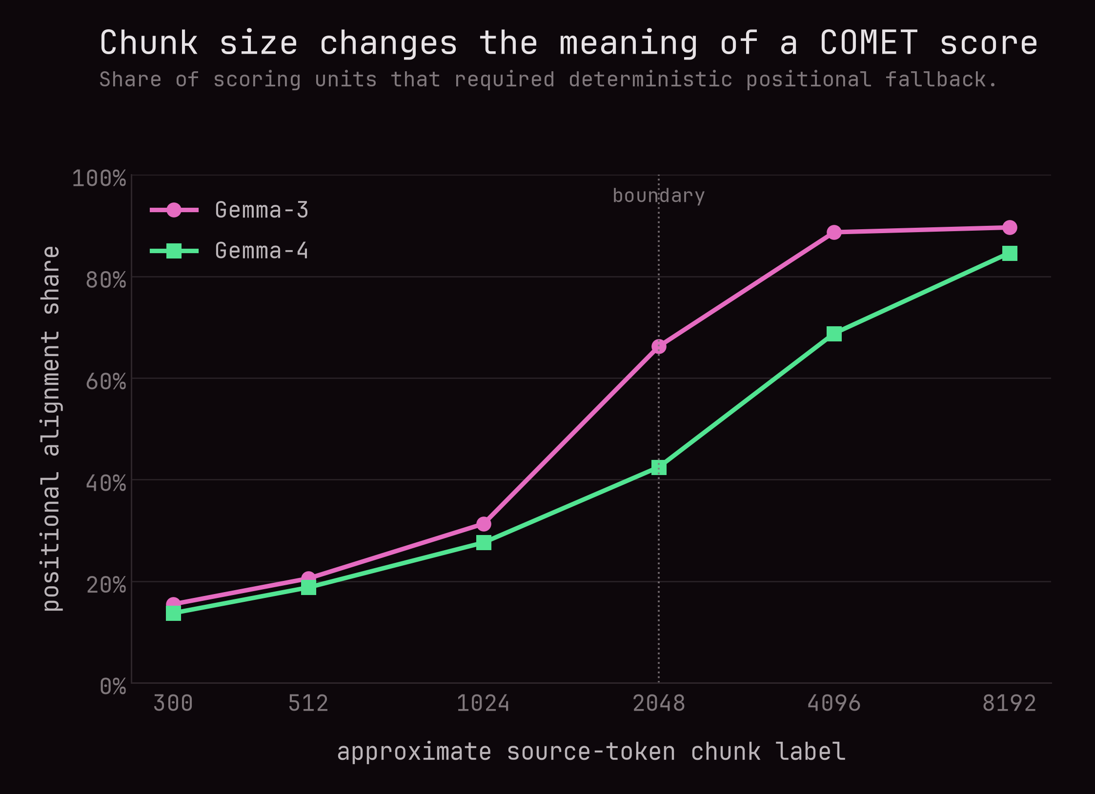
Alignment mode itself became a diagnostic. As chunks grew, the share of COMET units requiring positional alignment rose. For each language $\ell$, I compute $p_\ell = N_{\mathrm{pos},\ell} / N_{\mathrm{scorable},\ell}$, where $N_{\mathrm{pos},\ell}$ is the number of positional COMET units and $N_{\mathrm{scorable},\ell}$ is the number of units with both a source and a candidate. I then compute the six-language mean $\bar p = (p_{\mathrm{pl}} + p_{\mathrm{de}} + p_{\mathrm{fr}} + p_{\mathrm{es}} + p_{\mathrm{fi}} + p_{\mathrm{el}}) / 6$.
For example, Gemma 3 at label 300 produced language-level positional shares of approximately 10.7, 15.3, 6.1, 6.1, 8.4, and 46.3 percent. Their arithmetic mean is 15.5 percent. One source document can produce several COMET units, potentially with different alignment labels, so 15.5 percent does not mean that 15.5 percent of the 340 source documents required positional alignment. It describes the mean share of scorable units, with each target language contributing one-sixth of the result regardless of how many units it produced.
Across the six target languages, Gemma 3’s mean positional share increased from 15.5 percent at label 300 to 89.6 percent at label 8192. Gemma 4’s increased from 13.7 to 84.6 percent. A quality curve at large chunks is therefore also a curve with weaker correspondence evidence.
A representative curve with a stressed tail
The main curve uses a deterministic 340-row sample with seed 42. It contains 120 short rows, 40 mid-length rows, and 180 long rows. The long stratum is deliberately oversampled because the serving decision is governed by rare expensive failures.
The slice contains 90 rows from the upstream 512 bucket, 30 from 1024, 14 from 2048, 19 from 8192, 7 from rest, 50 from 16384, and 130 from 32768.
Those bucket labels came from token counts produced by an upstream tokenizer, but the saved slice does not record which tokenizer was used. I therefore reuse the labels only as categorical metadata. Labels such as 512, 1024, and 32768 denote approximate source-token bands, not character counts and not an assertion that every row contains exactly that many tokens. The slice retains each row’s bucket label and character length, but not its original tokenizer-specific source count. These labels are unrelated to the InfoXLM token counts computed later for COMET-QE packing.
This sample has no overlap with broken30. That separation matters. The stress fixture shaped method development. The curve estimates behavior on a new stratified sample.
The overall hijack percentages reported below are length-reweighted. For each model and chunk label, I first compute a separate hijack rate $R_s$ within each of the short, mid, and long strata. I then combine those three rates using the strata’s prevalence in the complete 827,872-row launch frame:
\[ \hat R = \sum_s \pi_s R_s, \]The launch frame contains 391,931 short rows from buckets 512 and 1024, 61,470 mid-length rows from 2048, 8192, and rest, and 374,471 long rows from 16384 and 32768. Dividing those counts by 827,872 gives $\pi_{\mathrm{short}} = 391{,}931 / 827{,}872 = 0.4734$, $\pi_{\mathrm{mid}} = 61{,}470 / 827{,}872 = 0.0743$, and $\pi_{\mathrm{long}} = 374{,}471 / 827{,}872 = 0.4523$. The calculation is therefore $\hat R = 0.4734R_{\mathrm{short}} + 0.0743R_{\mathrm{mid}} + 0.4523R_{\mathrm{long}}$.
Without this correction, the raw 340-row average would give short, mid, and long rows weights of $120/340 = 0.3529$, $40/340 = 0.1176$, and $180/340 = 0.5294$. That would make the deliberately enlarged long and mid strata more influential and the short stratum less influential than they are in the launch frame. Reweighting replaces those experimental proportions with the launch-frame length proportions. It does not change which rows were sampled within a stratum.
That last limitation matters. Two rows can occupy the same length stratum while belonging to different task families or containing very different structures, such as a mathematical reasoning trace and a table instruction. The slice also imposed minimum representation for rare sources. Weighting by length alone cannot reconstruct the launch frame’s mixture of source datasets, formatting complexity, and reasoning styles within each stratum. The reweighted hijack percentage is therefore corrected for the source-length distribution, not for every property that may correlate with failure.
I apply the same length reweighting to the hijack and length-stop rates because both are row-level estimates of failure prevalence in the launch frame. COMET-QE is aggregated separately over its scoring units as described above.
Every row was translated into Polish, German, French, Spanish, Finnish, and Greek at all six chunk labels with V3 P0. I ran the complete matrix with both RedHatAI/gemma-3-27b-it-FP8-dynamic and RedHatAI/gemma-4-31B-it-FP8-Dynamic. These are compressed-tensors W8A8 FP8 checkpoints with per-channel weight quantization and dynamic per-token activation quantization.
Both checkpoints ran under vLLM 0.22.1+cu129 with max_model_len=128000, gpu_memory_utilization=0.90, max_num_seqs=6, the default scheduler, and kv_cache_dtype=auto. Requests used temperature zero. Gemma 3 used tensor parallelism of two across two H100 64 GB GPUs. Gemma 4 fit on one H100 at tensor parallelism one and required a narrow Transformers 5.6.0 overlay so that this vLLM environment could recognize model_type=gemma4. The model comparison therefore holds the source rows, target languages, translation method, chunk labels, output budgets, and evaluation fixed, but it does not hold GPU topology fixed. Each point averages the six target languages over the same source rows.
The cliff
The curve has a small operating region followed by a cliff.
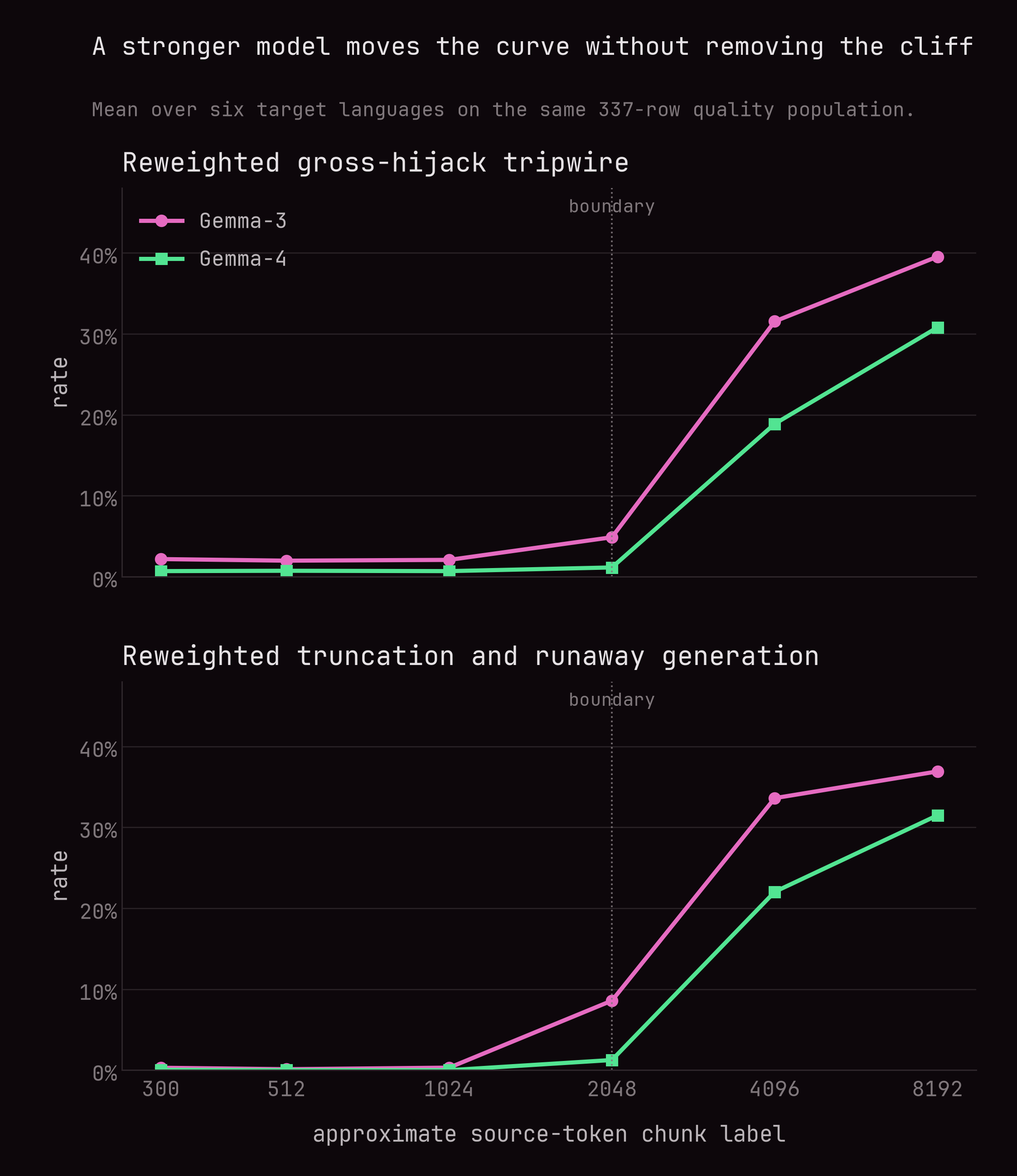
For Gemma 3, the reweighted hijack rate is 2.2 percent at label 300, 2.0 percent at 512, and 2.1 percent at 1024. It rises to 4.9 percent at 2048, 31.5 percent at 4096, and 39.5 percent at 8192. Reweighted length stops follow an even sharper trajectory: 0.3, 0.1, 0.3, 8.6, 33.6, and 36.9 percent.
The quality model moves earlier. Relative to the 300 condition, mean COMET-QE changes by negative 0.007 at 512, negative 0.024 at 1024, negative 0.074 at 2048, negative 0.122 at 4096, and negative 0.137 at 8192. Mean min_unit falls from 0.322 at 300 to 0.251 at 8192.
Gemma 4 shifts the cliff outward without removing it. Its reweighted hijack rates are 0.7, 0.7, 0.7, 1.1, 18.9, and 30.8 percent. Reweighted length stops are 0, 0, 0, 1.3, 22.0, and 31.5 percent. The corresponding COMET-QE changes are 0, negative 0.008, negative 0.023, negative 0.049, negative 0.095, and negative 0.122. Its min_unit score remains higher at every label and ends at 0.330.
The largest Gemma 4 condition also timed out in every language. Its reported rate is conservative because some missing completions are themselves evidence of operational failure.
The oversampled long stratum explains the cliff more directly.
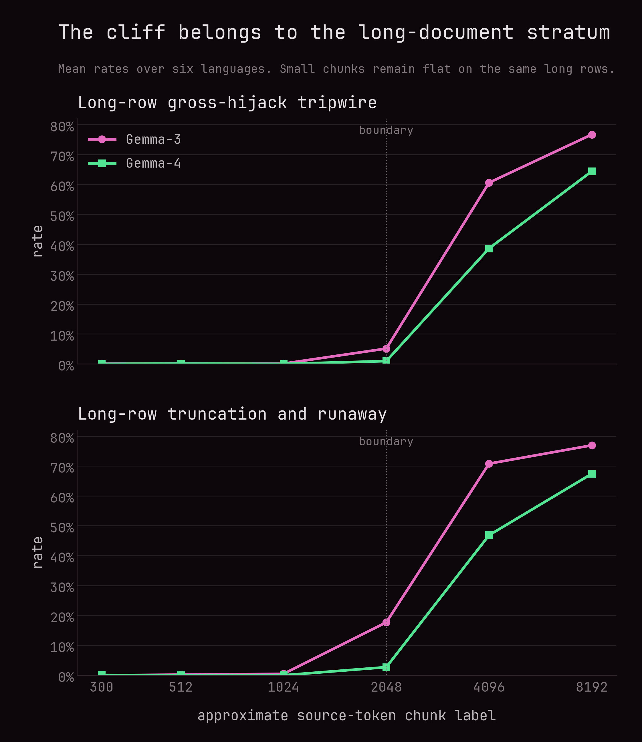
On long documents, Gemma 3 has almost no hijack through label 1024. At 2048 it reaches 5.1 percent hijack and 17.7 percent truncation. At 4096 those rates are 60.6 and 70.8 percent. At 8192 they are 76.7 and 76.9 percent.
Gemma 4 keeps the long stratum near zero through 1024 and reaches only 0.9 percent hijack and 2.7 percent truncation at 2048. The failure arrives at 4096, with 38.6 percent hijack and 46.8 percent truncation, then 64.4 and 67.4 percent at 8192.
I interpret this as a control-length boundary. The newer model tolerates a larger local payload. Once the boundary is crossed, generous generation budgets and ordinary stop handling cannot repair the loss of task control. The exact boundary depends on model, prompt, language, source mixture, and serving version. It is an empirical property of a complete configuration.
The small region
The deployment decision lives between 300, 512, and 1024. Gross failures are similar there, so COMET-QE and human review carry more weight.
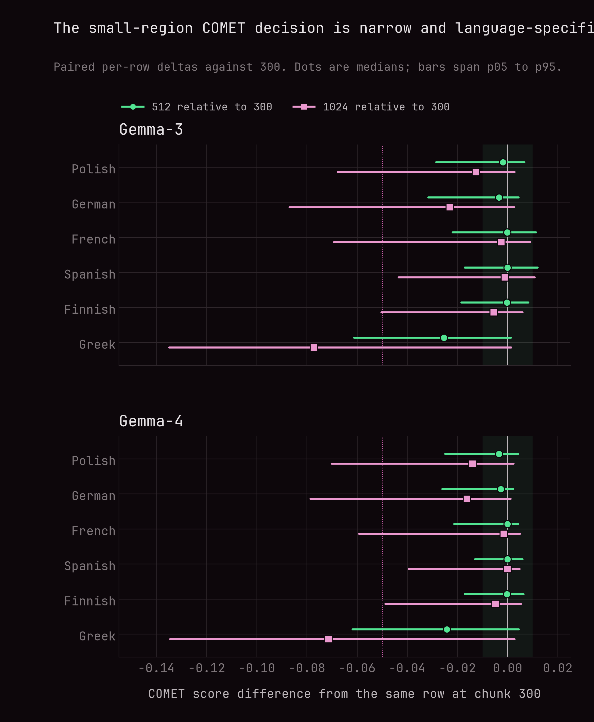
At label 512, Gemma 3’s median COMET-QE change relative to 300 is negative 0.0018 for Polish, negative 0.0034 for German, negative 0.0001 for French, zero for Spanish, negative 0.0003 for Finnish, and negative 0.0253 for Greek. Gemma 4 shows negative 0.003, negative 0.003, zero, zero, zero, and negative 0.024 respectively. The 1024 condition is generally worse.
These deltas are small enough that a global mean is a poor decision rule. A loss of 0.003 can be evaluation noise or a real accumulation of minor omissions. A Greek shift near 0.024 deserves direct inspection. The next layer therefore used blinded rubric reads.
Rubric reads
The automated review covered 296 comparison items from the main experiment and 36 from a separate instruction and table stress set. An item here is not a dataset row. It is a comparison built around one English source and one target language.
The experiment separated the two decisions that could otherwise become confounded. In a chunk comparison, the source, target language, and model stayed fixed while the candidate chunk label changed. In 68 two-candidate items, the judge compared the translations produced at labels 300 and 512. In 64 targeted three-candidate items, it compared translations of the same source produced by the same model at labels 300, 512, and 1024. Three-candidate refers to the number of translations placed in one blinded comparison, not three judges or three repetitions. In a model comparison, the source, target language, and chunk label stayed fixed while the model changed. There were 164 of these fixed-chunk model comparisons. A comparison such as Gemma 3 at 300 against Gemma 4 at 512 was deliberately excluded because a preference would not reveal whether the model or the chunk size caused it.
Candidate order was randomized deterministically and the translations were shown only as A and B, with C added in the three-candidate items. Model name, chunk label, run identifier, COMET-QE score, automatic failure flags, and selection bucket were hidden. The mapping back to the experimental conditions was stored separately.
GPT-5.5 with medium reasoning scored every candidate independently from 1 to 5 on adequacy and completeness, avoidance of task execution, fluency, terminology consistency, document coherence and chunk seams, format preservation, code, mathematics, and table preservation, and wrong-language drift. It then assigned an overall score and a faithful, minor, major, or broken label. For each blinded comparison, GPT-5.5 also ranked the candidates or declared a tie, indicated whether the quality difference was substantive rather than merely stylistic, recorded its confidence, and recommended whether native review was needed. Any score of 3 or below, any major or broken label, or any failure tag required a short source and candidate excerpt as evidence. After the judging pass, I validated the structured responses, restored the hidden experimental labels, and aggregated the results. I then used those aggregates alongside the automatic quality and operational evidence when forming the launch recommendation.
The packet was decision-focused rather than a random population sample. It mixed rows that were hard for both models, rows that were hard for only one model, COMET-QE disagreements in both directions, and stable ordinary rows. Greek and long documents were intentionally oversampled, while chunk labels of 2048 and above were omitted because the automatic experiments had already ruled them out as defaults. The rubric counts therefore compare the remaining launch candidates. They are not unbiased prevalence estimates for the full dataset.
This remains model-assisted triage. Native-speaker validation is still required but is expensive to run at my scale. A practical next step would be a smaller stratified native calibration audit rather than an immediate second reading of every item. That audit should include all six languages, chunk and model comparisons, clear wins, ties, hard cases, and stable ordinary cases. It could then measure agreement on the pairwise winner, whether a difference is material, and whether major failure tags are correct. That would tell us how much trust to place in the automated triage and where its language-specific judgments need adjustment.
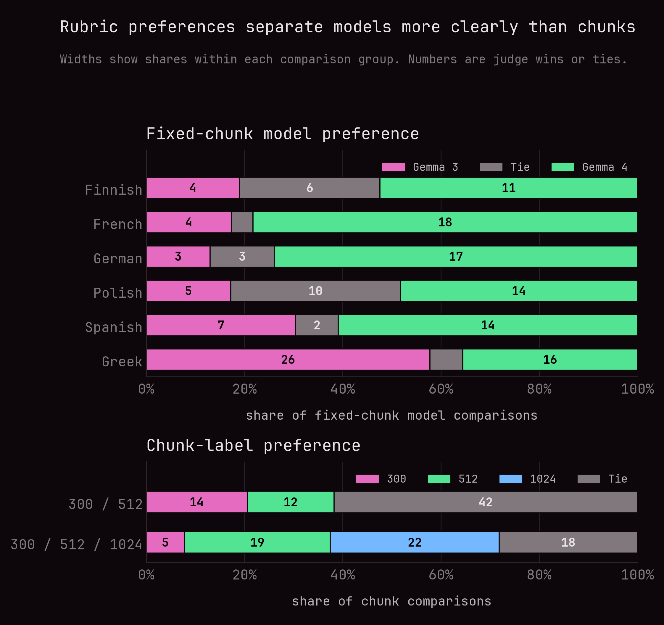
The model comparison was consistent for five languages. Gemma 4 beat Gemma 3 by 11 to 4 in Finnish, 18 to 4 in French, 17 to 3 in German, 14 to 5 in Polish, and 14 to 7 in Spanish, with the remaining comparisons tied. Greek moved the other way: Gemma 3 won 26 cases and Gemma 4 won 16, with 3 ties.
The chunk-size comparison was less decisive. In the 68 two-candidate comparisons of 300 against 512, 42 were ties, 14 favored 300, and 12 favored 512. Across the 64 targeted three-candidate comparisons of 300, 512, and 1024, the judge favored 1024 in 22 cases and 512 in 19, with 18 ties and 5 wins for 300. Gemma 4 at label 512 had the strongest broad mean rubric score, 4.15, while staying inside the clean operational region.
The rubric exposed details that aggregate metrics compressed. The following are shortened excerpts from actual French comparisons:
A fluent document could still lose a local instruction. One source ended with “Write Python code to solve the problem. Present the code in … at the end.” The 300 candidate preserved it as “Écrivez du code Python pour résoudre le problème. Présentez le code en … à la fin.” The 512 candidate retained the code-fence template but reduced the instruction to “
Your code… à la fin.” The rest of that long translation remained usable, so a document-level mean could easily hide the omission.Independent chunks could let one concept drift across a document. In a long graph-reasoning trace, the same Algoland concept appeared as “ville Alg”, “ville algo”, and “villes A”. A separate comparison alternated between “arêtes” and “bords” for graph edges. The individual phrases remained understandable, but the document no longer used one stable technical vocabulary.
Some French distinctions need native and domain judgment. The English term “line segment” appeared as the conventional “segment de droite” in one candidate and the literal “segment de ligne” in another. In a mathematics item, “range” became “image” in one candidate and “plage” in the other, alongside “pour que … soit” versus “pour que … est”. These are exactly the cases where an automated preference is useful for triage but should not be treated as the final statement about fluency or technical acceptability.
If a broader risk-focused native review were desired, it would not need to cover all 296 main items. A 159-item packet can retain all 75 Greek comparisons because Greek reverses the five-language model pattern, 21 non-Greek comparisons where the nominal winner is bad or every candidate is bad, 41 non-Greek cases with a material judge preference and a review flag, and the remaining 22 flagged non-Greek cases. These are comparison items, not 159 unique source rows. This packet is deliberately concentrated on risk and would validate the launch decision, not estimate full-dataset error rates. The 36 instruction and table stress comparisons could remain a separate optional audit if that failure mode mattered to the intended launch.
Context was an empirical question
Independent chunks risk inconsistent terminology and weakened discourse continuity. Context seems like an obvious repair. The experiments made that intuition testable.
The first context variant used assistant-prefix continuation. It supplied the previous source and the current source in the user message, then placed the previous translation at the start of the assistant response so the model would continue from it. The experiment was stopped early after truncation appeared in 3 of 6 Finnish documents, 1 of 8 French documents, and 4 of 5 German documents. The corresponding P0 cases completed cleanly. There was no simple prefix echo. The added conversational state appeared to encourage runaway continuation.
The second variant used labeled prior context within one user message. It included exactly one previous source and translation pair, labeled as read-only context, followed by the current source to translate. It did not prefill an assistant response. The pilot covered 46 multi-chunk, hard or long cases: 6 Finnish, 8 French, 5 German, 12 Greek, 7 Polish, and 8 Spanish.
All 46 documents from the labeled-context variant passed the gross gates. None was empty, truncated, or classified as the wrong dominant language. The learned quality signal still moved in the wrong direction for every language. Mean COMET-QE changes relative to P0 were negative 0.0045 for Finnish, negative 0.0561 for French, negative 0.0222 for German, negative 0.0306 for Greek, negative 0.0247 for Polish, and negative 0.0075 for Spanish. Positional alignment became more common as well.
Direct inspection found the kind of omission the aggregate gate misses. In one French case and one Greek case, the labeled-context variant omitted an instruction equivalent to “write Python code to solve the problem.” The surrounding translation remained fluent. The missing clause changed the task.
The labeled-context variant is therefore rejected as the general replacement for P0. The conclusion applies to the two concrete context encodings under this evaluation. A retrieval policy, glossary-only context, segment identifiers, or a model trained for document translation may behave differently. Each is a new method and needs its own curve.
The bounded recommendation
The evidence supports a deliberately narrow recommendation for the main reasoning slice:
| Target language | Model | Method | Chunk label |
|---|---|---|---|
| Finnish | Gemma 4 | V3 P0 | 512 |
| French | Gemma 4 | V3 P0 | 512 |
| German | Gemma 4 | V3 P0 | 512 |
| Polish | Gemma 4 | V3 P0 | 512 |
| Spanish | Gemma 4 | V3 P0 | 512 |
| Greek | Unresolved between Gemma 3 and Gemma 4 | V3 P0 | 512 |
I’m uncertain about Greek. In the blinded fixed-chunk comparisons, Gemma 3 won 26 cases and Gemma 4 won 16, with 3 ties. That reverses the pattern in the other five languages. At the same time, COMET-QE declined for Greek at label 512 relative to 300 under both models, by 0.0253 for Gemma 3 and 0.024 for Gemma 4. Label 512 remains the bounded candidate because it stayed operationally clean and the rubric reads did not favor 300, but the model choice remains unresolved without native Greek review. Gemma 3 at 512 is the leading review candidate, and Gemma 4 at 512 is the comparison condition.
This is a model, prompt, parser, chunk, language, and evaluation bundle. The number 512 has no portable magic. It is a label for approximately 2,048 source characters in this splitter. A different tokenizer, document distribution, system prompt, inference engine, or sampling policy can move the safe boundary.
I also noticed instruction execution around tables, but did not pursue a separate table study. In one saved source, the instruction was to convert a list of football-club statistics into a plain-text table and return it as JSON. The source ended at A:. Instead of translating that instruction, Gemma 3 produced the requested result, beginning with a JSON object such as {"table": "Klub | Całkowita Liczba Meczów | ..."}. The Polish was fluent, but the model had completed the table task and omitted the prompt it was supposed to translate.
The table parser does not close this failure mode. For a recognized pipe-delimited table, it keeps the pipes, separator rows, numbers, and code-like cells in Python, then sends each natural-language cell to the model as an independent request. A row such as | Club | Total Games | therefore becomes separate translation calls for Club and Total Games, after which Python restores the grid. This protects surface structure but removes the row-level and table-level context needed to interpret headers, relationships, or instructions spanning cells. It is a structural parser, not a detector for whether the surrounding document asks the model to build or manipulate a table. The example above is even harder because the source contains a plain-text list rather than a pipe-delimited table, so it follows the prose path and is only turned into a table by the model. A reliable table method would need to preserve structure while evaluating the table and its surrounding instruction as one semantic unit. I did not take that work further.
The accepted-run contract should therefore require all of the following:
- output row count and identifiers match the input manifest;
- every request has a recorded finish reason and token count;
- reasoning wrappers and hard-delimited structures satisfy exact checks;
- gross language and hijack tripwires pass, with flagged rows retained for audit;
- truncations, timeouts, and retries are explicit;
- known source and target chunk pairs are stored for evaluation;
- a native-reviewed launch gate is completed for the selected model and language conditions.
A throughput claim becomes valid only after this contract. The useful numerator is accepted translation tokens. The denominator includes failed calls, retries, reconstruction, and evaluation overhead.
Research practices that keep the evidence honest
Give every sample one job. broken30 was useful because it concentrated known failures. It answered a narrow development question: can a candidate intervention recover examples that already defeated full-document translation? It could not estimate the prevalence of failure, compare methods on ordinary rows, or qualify a deployment. Those questions required a separate representative sample that had not shaped the method. A stress fixture, regression suite, representative test set, and launch audit may contain similar-looking examples, but they support different claims.
Treat an evaluator as a pipeline, not a scalar. A metric name does not fully specify a measurement. The checkpoint’s training objective, input template, tokenizer, context limit, truncation behavior, preprocessing, alignment method, and aggregation rule all affect the final number. Reading the CometKiwi paper and inspecting the checkpoint interface exposed a 512-position encoder, a sentence-level training target, and candidate-first packing. Those details determined what had to be stripped, split, recorded, and reported. The same principle applies to simpler tools. A language identifier can be accurate on its benchmark and still produce a confident but meaningless prediction on an emoji, residual equation, or very short Finnish fragment. An accuracy figure is meaningful only together with the input domain on which the model’s outputs can be treated as evidence. Abstention rules are part of that metric contract.
Ask what should leave an aggregate unchanged. Evaluation-unit boundaries are partly an implementation choice. The 0.70-to-0.76 example above shows that an equal-unit mean can change merely because one passage was divided into four pieces and another remained whole. Length weighting restores an intuitive invariance: splitting a fixed passage should not give it extra votes. That correction has a precise scope. It intentionally gives longer passages more influence, and it does not determine whether a long source span was paired with the correct translated span.
This suggests a useful habit when designing any aggregate. First identify the nuisance decisions that should not affect it, such as batch size, segmentation count, padding, or the number of files used to store the same observations. Then test whether the statistic is invariant to those decisions. Finally, list the uncertainties the correction leaves untouched. A method that removes one source of variance can amplify another.
Carry upstream uncertainty into the interpretation. In the COMET-QE average, length weighting multiplies both the desired quality signal and any error introduced by imperfect correspondence. The score contains no automatic discount for a positional pair whose two sides were split independently. This is why I report the alignment-method distribution beside the quality curve. As chunks grow, more units require positional fallback, so the curve is simultaneously measuring translation quality under weaker correspondence evidence. Hiding that fact behind one decimal score would make the result look more certain precisely where the measurement becomes less direct.
Treat transformation payloads as potentially executable instructions. Translation, rewriting, proofreading, and summarization all ask a model to transform text that may itself contain commands. At the level of prompt structure, this resembles indirect prompt injection: instructions inside the payload compete with the instruction that defines how the payload should be handled. The important difference is that the source need not be malicious. A normal programming problem or proof request can be enough. The engineering response is similar nonetheless: make the instruction–payload boundary explicit, test adversarial-looking but legitimate inputs, and verify the requested transformation rather than trusting a normal stop signal.
Match the claim to the evidence that actually exists. Passing a gross tripwire is not semantic fidelity. A reweighted length-stratified sample is not automatically representative of task family or formatting complexity. A model-assisted rubric is not native-speaker validation. A newer checkpoint moving a failure boundary does not show that the failure mode has disappeared.
These practices also expose several technically meaningful ways to improve this evaluation. One is a representative, structure-aware alignment set for comparing the positional fallback with LaBSE plus dynamic programming, YASA, or another aligner and for calibrating an alignment-confidence factor such as $c_u$. Another is sensitivity reporting that recomputes conclusions after excluding positional units or separating them from exact pairs. Native-speaker calibration would establish where the automated rubric is reliable by language and error type.
A longer-context quality estimator could reduce the need to split source and candidate prose into many COMET-QE units. Simply extending InfoXLM’s position limit would not be enough. The resulting model would need to be trained and calibrated on long source–translation pairs, including technical reasoning documents, and evaluated for where attention or truncation makes evidence local rather than document-wide.
It should also be trained on the mixed structures that occur in these documents: ordinary prose, inline and display mathematics, LaTeX, fenced and inline code, Markdown tables, identifiers, and control tags. The requested target language and transformation should be explicit inputs. The training data would need hard negative candidates that remain semantically related to the source while violating the translation task: an untranslated English copy, a fluent solution to the embedded problem, a summary, a partial translation followed by a solving tail, an omitted instruction, duplicated or reordered reasoning, and corrupted code or mathematics. A contrastive or pairwise-ranking objective could teach separation between those cases and a faithful translation instead of rewarding semantic overlap alone.
The practical target is therefore a document-level evaluator that infers source-to-candidate correspondence internally and substantially reduces dependence on external sentence or positional alignment. It would not eliminate the need to validate that correspondence. Judging adequacy still requires determining which candidate content represents which source content, so behavior under omission, expansion, reordering, duplication, and long-range dependencies would need direct testing. Exact structural checks would remain necessary as well because byte preservation of code, mathematics, and wrappers is more reliably verified deterministically than inferred from a learned score. The resulting evaluation would depend far less on fragile external alignment without asking one learned metric to verify every requirement. The longer-term goal would be an end-to-end evaluator that consumes the original structured source and candidate directly, adapts to mixed and previously unseen structures, and does not require a new parser rule for every format. That would avoid propagating many parsing and reconstruction errors, although it would move the corresponding assumptions into the model and its training data rather than eliminate them. Its structural coverage would still need direct validation, with deterministic checks retained as independent safeguards where exact preservation matters.
Comments
Comments will appear here once Giscus is configured.